ADVANCED DIPLOMA IN MANAGEMENT

ECONOMICS

ADVANCED DIPLOMA IN

MANAGEMENT

ECONOMICS

MODULE GUIDE

REGENT BUSINESS SCHOOL

photocopying machines, without the written permission of the publisher.

ADVANCED DIPLOMA IN MANAGEMENT

ECONOMICS

Table of Contents

INTRODUCTION TO ECONOMICS ............................................................................... 3

CHAPTER 1:

Economic Systems ......................................................................................................... 8

CHAPTER 2:

Characteristics of Competitive Environments ............................................................... 98

CHAPTER 3:

Main Economic Policies ............................................................................................. 177

BIBLIOGRAPHY ........................................................................................................ 203

ADVANCED DIPLOMA IN MANAGEMENT

ECONOMICS

List of Tables and Figures

Figure 1.1: An example of a Production Possibilities Frontier (PPF) .............. 17

Figure 1.2.1: PPF & Marginal Costs highlighting allocative efficiencies ......... 19

Figure 1.2.2: PPF & Marginal Costs highlighting allocative efficiencies ......... 19

Figure 1.3: Economic Circular Flows .............................................................. 23

Figure 1.4: Demand Curve ............................................................................. 26

Figure 1.5: Price of related goods .................................................................. 27

Figure 1.6: Expected future prices ................................................................. 28

Figure 1.7: Increase in income ....................................................................... 29

Figure 1.8: Expected future income................................................................ 29

Figure 1.9: Population and demand .............................................................. 30

Figure 1.10: Preferences ................................................................................ 31

Figure 1.11: Change in the quantity demanded versus a change in demand. 32

Figure 1.12: Determining the price, quantity, income of factors of production 34

Figure 1.13: The effect of a shift of the demand curve ................................... 36

Figure 1.14: A change in quantity supplied versus a change in supply……… 37

Figure 1.15: Market equilibrium ...................................................................... 38

Figure 1.16: Changes in supply ...................................................................... 40

Figure 1.17: Categories of Price Elasticity of Demand ................................... 42

Figure 1.18: Total welfare - combined consumer & producer surplus ............ 52

Figure 1.19: Deadweight Loss from minimum wage....................................... 57

Figure 1.20: Effects of a tax on supply (sellers) ............................................. 59

Figure 1.21: Effects of a tax on demand (buyers) .......................................... 59

Figure 1.22: Perfectly price inelastic demand ................................................. 60

Figure 1.23: Perfectly price elastic demand) .................................................. 61

Figure 1.24: International Markets in Action ................................................... 65

Figure 1.25: Consumption Possibility Budget Line ......................................... 72

Figure 1.26: Paradox of value ........................................................................ 78

Figure 2.1: Product curve graph ..................................................................... 111

Figure 2.2.: Marginal Product Curve .............................................................. 112

Figure 2.3.: Average Product Curve ............................................................... 113

Figure 2.4.: The cost curve effect on production ............................................ 116

Figure 2.5.: Short-run supply curve ................................................................ 121

ADVANCED DIPLOMA IN MANAGEMENT

ECONOMICS

Figure 2.6.: The firm’s short-run shut-down decision...................................... 124

Figure 2.7.: Long-run supply curve ................................................................. 126

Figure 2.8.: Cost of Monopoly ........................................................................ 132

Figure 2.9.: Monopolistic competition in the short run .................................... 138

Figure 2.10.: Monopolistic competition in the long run ................................... 139

Figure 2.11: Oligopoly and Demand ............................................................... 141

Figure 2.12: Equilibrium Employment in a Competitive Labour Market .......... 145

Figure 2.13: Firm’s labour Demand Curve ..................................................... 148

Figure 2.14: An Individual’s Labour Supply Curve ......................................... 149

Figure 3.1: Laffer Curve .................................................................................. 184

Table 1.1: Maximising Utility ........................................................................... 74

Table 1.2: Marginal Utility per rand ................................................................ 76

Table 2.1: Marginal Revenue Product of Labour ............................................ 147

ADVANCED DIPLOMA IN MANAGEMENT

ECONOMICS

INTRODUCTION TO ECONOMICS

1. Introduction

Welcome to the Advanced Diploma in Management programme. As part of your

studies, you are required to study and successfully complete a course on

Economics.

2. Module Overview

Economics plays a role in our everyday life. By studying economics, it enables us to

understand past, future, and current economic models, and apply them to societies,

governments, businesses, and individuals. Economics uses scientific methods to

understand how scarce resources are exchanged within society. These can be

individual decisions, family decisions, business decisions or societal decisions.

Scarcity is a fact of life. Scarcity means that human wants for goods, services and

resources exceed what is available. Resources, such as labour, tools, land, and raw

materials are necessary to produce the goods and services we want but they exist in

limited supply. Of course, the ultimate scarce resource is time. Everyone, rich or

poor, has just twenty-four hours in the day to try to acquire the goods that they want.

At any point, there is only a finite number of resources available. Because these

resources are limited, so are the numbers of goods and services we produce with

them. Combine this with is the fact that human “wants” are virtually infinite. In this

module we will be discussing how market works, the impact of household choices

and the role of firms and markets in this. We will look at the different market failures

and governments response, factor markets, inequality and uncertainty, and the role

of governments in macro-policy development.

3. Aim of the Module

At the end of the module the student would be able to:

• Demonstrate an understanding of basic economic principles and concepts

ADVANCED DIPLOMA IN MANAGEMENT

ECONOMICS

• Distinguish between the various economic systems

• Elaborate on the concepts of supply and demand

• Illustrate the various forms of elasticity

• Discuss the types of unemployment and outline policies to combat

unemployment

• Discuss the concept of inflation and describe the tools that may be utilised

combat the effects of inflation

4. Essential (Prescribed) Reading

Your essential (prescribed) reading comprises the following:

4.1. Prescribed Reading

Parkin M, Kohler M, Lakay L, Rhodes B, Saayam A, Schoer V, Scholtz F,

Thompson K. (2019). Economics: Global and Southern African Perspectives.

3rd Edition. Pearson Education South Africa.

4.2. Recommended Reading

Harford, T (2007). The Undercover Economist. Random House. 3rd Edition.

USA.

5. How to use the Module

This module should be studied using the recommended and prescribed textbook/s in

conjunction with the relevant sections of this module. You must read about the topic

that you intend to study in the appropriate section before you start reading the

textbook/s in detail. Ensure that you make your own notes as you work through both

the textbook/s and this module. You will find a list of objectives and outcomes at the

beginning of each section. These outline the main points that you need to

understand when you have completed the section/s. The purpose of this guide is to

help you study. It is important for you to work through all the tasks and self-

assessment exercises as they provide guidelines for examination purposes.

ADVANCED DIPLOMA IN MANAGEMENT

ECONOMICS

6. Navigational Icons

Think Point

When you see this icon, you should think about and reflect on the

issues/challenges/themes presented.

Tasks

When you see this icon, you will know that you are required to

perform some kind of task to gauge how well you remember or

understand what you have read or how good you are at applying

what you have learnt.

Key Words and Definitions

This icon will alert you to a specific definition related to the topic

under discussion

Case Studies

Case studies are often used to illustrate a concept within the setting

of a real-life scenario. Answer the questions that follow to ensure

that you have a proper understanding of what has been discussed.

7. Specific Outcomes and Chapter Alignment

SPECIFIC PROGRAMME OUTCOMES

CHAPTER

ALIGNMENT

SO1:

Solve basic economic problems in different

economic systems.

Chapter 1

SO2:

Distinguish between the characteristics of the

various competitive environments.

Chapter 2

SO3:

Demonstrate an understanding of the main

economic policies.

Chapter 3

ADVANCED DIPLOMA IN MANAGEMENT

ECONOMICS

8. Specific Outcomes and Assessment Criteria

SPECIFIC PROGRAMME

OUTCOMES

ASSESSMENT CRITERIA

The student should demonstrate the

ability to:

SO1:

Solve basic economic

problems in different

economic systems.

• Apply and evaluate key terms,

concepts of supply and demand

whilst simultaneously considering

the impact of the forms of elasticity.

• Understand and be able to evaluate

knowledge scopes of competitive

environments and inflation.

• Identify, analyse, evaluate, critically

reflect on, and address complex

unemployment and related

problems, applying evidence-based

solutions and theory-driven

arguments when it comes to policy

development.

SO2:

Distinguish between the

characteristics of the various

competitive environments.

SO3:

Demonstrate an

understanding of the main

economic policies.

ADVANCED DIPLOMA IN MANAGEMENT

ECONOMICS

CHAPTER 1:

Economic Systems

Chapter Outcome

Upon completion of this chapter, the learner should be able to:

• Understand and evaluate knowledge of competitive environments and inflation.

1.1. Introduction to Economic Systems

An economic system is a means by which societies or governments organise and

distribute available resources, services, and goods across a geographic region or

country. Economic systems regulate the factors of production, including land, capital,

labour, and physical resources. An economic system encompasses many

institutions, agencies, entities, decision-making processes, and patterns of

consumption that comprise the economic structure of a given community. In this

chapter we will therefore be going over the concepts that determine economics, how

a market works and the different role players, and the choices that are available to

households.

Key Words and Definitions

Bear market: The principle of a bear market is simple enough.

Essentially, it represents a negative or pessimistic outlook on a stock

market’s performance, often with such markets falling into a downfall

spiral, where prices continue to drop. As a result of a bear market,

selling of stocks tends to increase. Additionally, investors expect, and

Think Point

What type of economic system do you think applies to your country?

ADVANCED DIPLOMA IN MANAGEMENT

ECONOMICS

may well receive, increased losses from their investments.

Bond: This is a debt-based investment that represents a promise to

pay from the bond issuer; the bond issuer owes money to bond

investors on a certain date

Bull market: A bull market represents a much more positive outlook

on a stock market’s performance compared to a bear market. In a

bull market, stock prices either have or are expected to increase.

Capital goods: These are items a business uses to produce goods

or services to sell to consumers; examples include manufacturing

equipment and business facilities.

Commodity: These are raw materials (like crude oil or iron ore) or

agricultural product (like unprocessed wheat or corn) purchased in

enormous quantities for production purposes.

Consumer: This is anyone (person or business) that uses

(consumes) goods or services.

Demand: The extent to which there is a market for goods or

services; when a lot of people want to buy something, demand is

high.

Elasticity: This is how much an economic variable changes in

response to another; if demand spikes when prices are low but

contract when prices are high, that is elastic demand.

Elasticity of demand: This describes how the demand for goods or

services increases or decreases when the price of that good or

service changes. Goods that generally are susceptible to the

elasticity of demand should exhibit the following patterns, namely, an

increase in the cost of the good will lead to a decrease in demand,

whereas a decrease in the cost of the good will lead to an increase in

demand.

ADVANCED DIPLOMA IN MANAGEMENT

ECONOMICS

Equity: This is the amount of ownership in an asset; the equity a

person has in their home is the difference between the property’s

value and the amount owed on the mortgage.

Financial markets This refers to a market or marketplace where

financial assets are bought and sold. A common example of a

financial market is a stock exchange.

Leverage: This is the extent to which an investment is funded with

borrowed money (debt); the investor is relying on earning a return in

order to pay off the debt and still make a profit.

Liquidity: This is the extent to which assets could quickly be

converted to cash; for example, a checking account is more liquid

than a one-year certificate of deposit.

Law of demand: The law of demand examines how customers’

buying habits change when prices increase. Specifically, the theory

posits that all other things being equal, when prices of a good

increase, the demand for that good will fall.

Law of supply: The law of supply states that all other things being

equal, an increase in price levels results in an increase in the quantity

of those goods that are supplied.

Market: This is any means that buyers and sellers use to exchange

money for goods or services.

Marginal utility: This refers to the amount of satisfaction a consumer

has by consuming a good or service. Marginal utility can be used by

economists to gauge how much of a good or service a consumer

should buy.

Opportunity cost: This is the cost of missing an opportunity in order

to take on a different opportunity. An example of opportunity cost can

be seen in investors, who may have to forego investing in one

ADVANCED DIPLOMA IN MANAGEMENT

ECONOMICS

company in order to invest in another.

Scarcity: These are resources or products that aren’t available in

unlimited quantities are scarce; as scarcity of an item increases, so

do prices.

Shift in demand: This is when the demand for a product or service

goes up or down due to factors other than a change in price.

Supply: This determines how much is available of a particular good

or service; when supply of a product goes down, the item becomes

scarce.

1.2. Introducing Economics

Economics is the social science that studies the choices that individuals, businesses,

governments, and entire societies make as they cope with scarcity and the

incentives that influence and reconcile those choices. It consists of two parts, namely

microeconomics and macroeconomics.

• Microeconomics: This is the study of the choices that individuals and

businesses make, the way these choices interact in markets and the influence of

governments. Some examples of microeconomic questions are: Why are people

downloading more movies and TV series? How would a tax on e-commerce

affect takealot.com?

• Macroeconomics: This is the study of the performance of the national economy

and the global economy. Some examples of macroeconomic questions are: Why

is the South African unemployment rate one of the highest in the world? Can the

South African Reserve Bank make our economy expand by cutting interest rates?

1.2.1. Understanding our changing world

Two big questions summarise the scope of economics:

ADVANCED DIPLOMA IN MANAGEMENT

ECONOMICS

• How do choices end up determining what, how and for whom goods and

services are produced?

• When do choices made in the pursuit of self-interest also promote the social

interest?

Goods and services: These are the objects that people value and produce to

satisfy human wants. Goods are physical objects such as cell phones and cars.

Services are tasks performed for people such as those at cell phone repair centres

and car service centres.

Production choices: What we produce varies across countries and changes over

time. The largest part (two-thirds, in fact) of what South Africa produces today is

services, such as retail and wholesale trade, health care and education. Goods are a

small part of total production.

Factors of production: This is described by the technologies and resources that we

use, and is grouped into four categories, namely land, labour, capital, and

entrepreneurship.

1. Land

In economics, land is what in everyday language we call natural resources. It

includes land in the everyday sense of the word together with minerals, oil, gas, coal,

water, air, forests, and fish. Our land surface and water resources are renewable and

some of our mineral resources can be recycled. But the resources that we use to

create energy, such as oil and coal, are non-renewable – they can be used only

once.

2. Labour

This is the work time and work effort that people devote to producing goods and

services. It includes the physical and mental efforts of all the people who work on

farms and construction sites and in factories, shops, and offices. The quality of

labour depends on human capital which is the knowledge and skills that people

obtain from education, on-the-job training, and work experience. One can build one’s

ADVANCED DIPLOMA IN MANAGEMENT

ECONOMICS

own human capital right now during the economics course, and one’s human capital

will continue to grow as work experience is gained.

3. Capital

These are the tools, instruments, machines, buildings, and other constructions that

businesses use to produce goods and services. Money, stocks, and bonds can also

be considered ‘capital’. These items are financial capital. Financial capital plays an

important role in enabling businesses to borrow the funds that they use to buy

capital. But financial capital is not used to produce goods and services, nor is it a

factor of production.

4. Entrepreneurship

This is the human resource that organises labour, land, and capital. They develop

new ideas about what and how to produce, make business decisions and bear the

risks that arise from these decisions.

The type of people that consume the different goods and services that are produced,

depends on the incomes that these different people earn. People with large incomes

can buy a wide range of goods and services. People with small incomes have fewer

options and can afford a smaller range of goods and services. People earn their

incomes by selling the services of the factors of production they own, such as:

• Land earns rent.

• Labour earns wages.

• Capital earns interest.

• Entrepreneurship earns profit.

Choices in the pursuit of self-interest and the promotion of social interest: All

the choices that people make about how to use their time and other resources are

made in the pursuit of self-interest, such as one’s time, budget and choices which

will influence how one feels about the choices made.

Social interest: An outcome is in the social interest if it is best for society as a

whole.

ADVANCED DIPLOMA IN MANAGEMENT

ECONOMICS

Efficiency and the social interest: Economists use the everyday word ‘efficient’ to

describe a situation that cannot be improved upon. Resource use is efficient if it is

not possible to make someone better off without making someone else worse off. If it

is possible to make someone better off without making anyone worse off, society can

be made better off, and the situation is not efficient.

Fair shares and the social interest: The idea that social interest requires "fair

shares" is deeply held. Fair shares do matter, but what is fair? People say that too

much inequality is unfair but how much is too much, and the inequality of what? Is it

income, or wealth, or the opportunity to work, to earn an income, and accumulate

wealth? There are four issues in today’s world that are related to these questions,

namely:

1. Globalisation

2. Information-age monopolies

3. Climate change

4. Economic instability

1. Globalisation

The term globalisation means the expansion of international trade, borrowing and

lending, and investment. While globalisation brings expanded production and job

opportunities for some workers, it destroys many domestic jobs. Workers across the

manufacturing industries must learn new skills, take service jobs, which often pay

less, or retire earlier than previously planned. Globalisation is in the self-interest of

those consumers who buy low-cost goods and services produced in other countries;

and it is in the self-interest of the multinational firms that produce in low-cost regions

and sell in high-price regions.

2. Information-age monopolies

The technological change of the past forty years has been called the Information

Revolution. The information revolution has clearly served one’s own self-interest; it

has provided tools such as smartphones, laptops, loads of handy applications, and

the internet. It has also served the self-interest of the owners of the companies that

supplied these goods.

ADVANCED DIPLOMA IN MANAGEMENT

ECONOMICS

3. Climate change

Every day, when a person makes self-interested choices to use electricity and petrol,

they contribute to their own carbon footprint, which can be lessened by walking,

riding a bike, taking a cold shower, or planting a tree – however, can each one of us

be relied upon to make decisions that affect the Earth’s carbon-dioxide concentration

in the social interest?

4. Economic instability

Banks’ choices to take deposits and make loans are made in self-interest, but does

this lending and borrowing serve the social interest? Do banks lend too much in the

pursuit of profit?

The questions that economics tries to answer tell us about the scope of economics,

but they do not tell us how economists think and go about seeking answers to these

questions, namely that:

1. A choice is a trade-off.

2. People make rational choices by comparing benefits and costs.

3. Benefit is what a person will gain from something.

4. Cost is what a person must give up in getting something.

5. Most choices are ‘how-much’ choices made at the margin.

6. Choices respond to incentives.

1. A choice is a trade-off

As we face scarcity, we must make choices. When we make a choice, we select

from the available alternatives. A trade-off is an exchange, to give up one thing, to

get something else.

2. People make rational choices by comparing benefits and costs

A rational choice is one that compares costs and benefits and achieves the greatest

benefit over cost for the person making the choice. Only the wants of the person

making a choice are relevant to determine its rationality.

ADVANCED DIPLOMA IN MANAGEMENT

ECONOMICS

3. Benefit is what a person will gain from something

The benefit of something is the gain or pleasure that it brings and is determined by

preferences, by what a person likes and dislikes and the intensity of those feelings.

Economists measure benefit as the most that a person is willing to give up getting

something.

4. Cost is what a person must give up in getting something

The opportunity cost of something is the highest-valued alternative that must be

given up getting it. It has two components: The things that a person cannot afford to

buy and the things that they cannot do with their time, such as the rand-value of that

time, or all the items that make up the opportunity cost. They involve choosing how

much of an activity to do.

5. Most choices are ‘how-much’ choices made at the margin

A person must decide how many minutes to allocate to each activity. The decision is

made at the margin. The benefit that arises from an increase in an activity is called

marginal benefit. The opportunity cost of an increase in an activity is called marginal

cost.

6. Choices respond to incentives.

The central idea of economics is that we can predict the self-interested choices that

people make by looking at the incentives they face. People undertake those activities

for which marginal benefit exceeds marginal cost; and they reject options for which

marginal cost exceeds marginal benefit. Economists see incentives as the key to

reconciling self-interest and social interest. When our choices are not in the social

interest, it is because of the incentives we face. One of the challenges for

economists is to figure out the incentives that result in self-interested choices being

in the social interest.

ADVANCED DIPLOMA IN MANAGEMENT

ECONOMICS

1.2.2. The Economic Problem

The quantities of goods and services that we can produce are limited both by our

available resources and by technology, if we want to increase our production of one

good, we must decrease the production of something else, we therefore face a

trade-off.

Figure 1.1. An example of a Production Possibilities Frontier (PPF)

Source: Creative Commons License

The production possibilities frontier (PPF): This is the boundary between those

combinations of goods and services that can be produced and those that cannot.

The PPF illustrates scarcity because we cannot attain the points outside the frontier.

These points describe wants that cannot be satisfied. We can produce at any point

inside the PPF or on the PPF, such as points A, B, C and D. F is attainable and is

inside the curve, but the products produced at this point would be wasted, or

misallocated, whereas E is outside the curve and not attainable

Production efficiency: We achieve production efficiency if we produce goods and

services at the lowest possible cost. This outcome occurs at all the points on the

PPF. Producing at any output level on the PPF implies the maximisation of

production given the available resources – hence the term production efficiency. At

points inside the PPF, production is inefficient because we are giving up more than

necessary of one good to produce a given quantity of the other good.

ADVANCED DIPLOMA IN MANAGEMENT

ECONOMICS

Trade-off along the PPF: Every choice along the PPF involves a trade-off. Trade-

offs arise in every imaginable real-world situation in which a choice must be made.

At any given point in time, we have a fixed amount of labour, land, capital, and

entrepreneurship. By using our available technologies, we can employ these

resources to produce goods and services but are limited in what we can produce.

This limit defines a boundary between what we can attain and what we cannot attain.

This boundary is the real world’s production possibilities frontier, and it defines the

trade-offs that we must make. On our real-world PPF, we can produce more of any

one good or service only if we produce less of some other goods or services.

Opportunity cost: The opportunity cost of an action is the highest-valued alternative

forgone. The PPF makes this idea precise and enables us to calculate opportunity

cost. Along the PPF, there are only two goods, so there is only one alternative

forgone: some quantity of the other good.

• Opportunity cost is a ratio It is the decrease in the quantity produced of one

good divided by the increase in the quantity produced of another good as we

move along the production possibilities frontier.

Using resources efficiently: We achieve production efficiency at every point on the

PPF, but which point is best? The answer is the point on the PPF at which goods

and services are produced in the quantities that provide the greatest possible

benefit. When goods and services are produced at the lowest possible cost and in

the quantities that provide the greatest possible benefit, we have achieved allocative

efficiency.

The PPF and marginal cost: The marginal cost of a good is the opportunity cost of

producing one more unit of it. We calculate marginal cost from the slope of the PPF.

Preferences and marginal benefit: The marginal benefit from a good or service is

the benefit received from consuming one more unit of it. This benefit is subjective. It

depends on people’s preferences – people’s likes and dislikes and the intensity of

those feelings. Marginal benefit and preferences stand in sharp contrast to marginal

cost and production possibilities. Preferences describe what people like and want

and the production possibilities describe the limits or constraints on what is feasible.

We measure the marginal benefit from a good or service by the most that people are

ADVANCED DIPLOMA IN MANAGEMENT

ECONOMICS

willing to pay. Below one can see the allocative efficiencies that are demonstrated in

graph A versus the marginal costs in graph B.

Product X

Amount Product Y Amount Product Y

Graph A - PPF Graph B – Marginal cost

Figure 1.2.1. PPF & Marginal Costs highlighting allocative efficiencies

Source: Creative Commons License

To highlight this further, the PPF and opportunity cost (a) and the marginal cost

demonstrated in (b) are shown in cooldrinks, versus hamburgers, as such:

Figure 1.2.2. PPF & Marginal Costs highlighting allocative efficiencies

Source: Parkin M, et al. (2019). Economics: Global and Southern African

Perspectives. 3rd Edition. Pearson Education South Africa.

ADVANCED DIPLOMA IN MANAGEMENT

ECONOMICS

Allocative efficiency: At any point on the PPF, we cannot produce more of one

good without giving up some other good. At the best point on the PPF, we cannot

produce more of one good without giving up some other good that provides greater

benefit. We are producing at the point of allocative efficiency which is the point on

the PPF that we prefer above all other points.

Economic growth: The expansion of production possibilities is called economic

growth. Economic growth increases our standard of living, but it does not overcome

scarcity and avoid opportunity cost. To make our economy grow, we face a trade-off,

which means that the faster we make production grow, the greater is the opportunity

cost of economic growth.

The cost of economic growth: Economic growth comes from technological change

and capital accumulation. Technological change is the development of new goods

and of better ways of producing goods and services. Capital accumulation is the

growth of capital resources, including human capital. Technological change and

capital accumulation have vastly expanded our production possibilities.

A nation’s economic growth: If a nation devotes all its factors of production to

producing consumption goods and services and none to advancing technology and

accumulating capital, its production possibilities in the future will be the same as they

are today. To expand production possibilities in the future, a nation must devote

fewer resources to producing current consumption goods and services and some

resources to accumulating capital and developing new technologies. As production

possibilities expand, consumption in the future can increase. The decrease in today’s

consumption is the opportunity cost of tomorrow’s increase in consumption.

Gains from trade: People can produce for themselves all the goods and services

that they consume, or they can produce one good or a few goods and trade with

others. Producing only one good or a few goods is called specialisation. It is

therefore the ability of two agents to increase their consumption possibilities by

specialising in the good in which they have comparative advantage and trading for a

good in which they do not have comparative advantage

Comparative and absolute advantage: A person has a comparative advantage in

an activity if that person can perform the activity at a lower opportunity cost than

ADVANCED DIPLOMA IN MANAGEMENT

ECONOMICS

anyone else. Differences in opportunity costs arise from differences in individual

abilities and from differences in the characteristics of other resources.

• Absolute advantage describes a situation in which an individual, business or

country can produce more of a good or service than any other producer with

the same quantity of resources.

• Comparative advantage describes a situation in which an individual,

business or country can produce a good or service at a lower opportunity cost

than another producer.

• Production specialisation according to comparative advantage, not absolute

advantage, results in exchange opportunities that lead to consumption

opportunities beyond the PPC. Trade between two agents or countries allows

the countries to enjoy a higher total output and level of consumption than what

would have been possible domestically.

Achieving the gains from trade: Comparative advantage and opportunity costs

determine the terms of trade for exchange under which mutually beneficial trade can

occur. The terms of trade refer to the trading price agreed upon by two agents, which

when beneficial, will allow both countries to enjoy gains from trade.

Economic coordination: People gain by specialising in the production of those

goods and services in which they have a comparative advantage and then trading

with each other. For billions of individuals to specialise and produce millions of

different goods and services, their choices must somehow be coordinated. Two

competing economic coordination systems have been used namely, central

economic planning and decentralised markets.

• Central economic planning was tried in Russia and China and is still used in

Cuba and North Korea. This system works badly because government

economic planners do not know people’s production possibilities and

preferences. Resources get wasted, production ends up inside the PPF and

the wrong things get produced.

• Decentralised (market) coordination works best but to do so it needs four

complementary social institutions. They are:

1. Firms.

2. Markets.

ADVANCED DIPLOMA IN MANAGEMENT

ECONOMICS

3. Property rights.

4. Money.

1. Firms

A firm is an economic unit that hires factors of production and organises those

factors to produce and sell goods and services. Firms coordinate a huge amount of

economic

activity. Firms specialise in providing a particular product or service. The trade

between firms takes place in (decentralised) markets.

2. Markets

A market is any arrangement that enables buyers and sellers to get information and

to do business with each other. A market is therefore a network of producers, users,

wholesalers and brokers, or buyers that buy and sell products and services. These

networks deal with each other through telephone, computer, and other methods.

Markets facilitate trade. Enterprising individuals and firms, each pursuing their own

self-interest, have profited from making markets by standing ready to buy or sell the

items in which they specialise. Markets can only work however, when property rights

exist.

3. Property rights

The social arrangements that govern the ownership, use and disposal of anything

that people value is called property rights. Real property includes land and buildings,

those things we call property and durable goods such as plant and equipment.

Financial property includes stocks and bonds and money in the bank. Intellectual

property is the intangible product of creative effort. This type of property includes

books, music, computer programs and inventions of all kinds and is protected by

copyrights and patents. Where property rights are enforced, people have an

incentive to specialise and produce the goods in which they have a comparative

advantage. Where people can steal the production of others, resources are devoted

not to production but to protecting possessions.

ADVANCED DIPLOMA IN MANAGEMENT

ECONOMICS

4. Money

Money is any commodity or token that is generally acceptable as a means of

payment. Trade in markets can exchange any item for any other item. However, the

use of money makes trading in markets much more efficient.

Figure 1.3. Economic Circular Flows

Source: Creative Commons License

Circular flows through markets: There are the flows that result from the choices

that households and firms make. Households specialise and choose the quantities of

labour, land, capital, and entrepreneurial services to sell or rent to firms. Firms

choose the quantities of factors of production to hire. These flows go through to the

factor markets. Households choose the quantities of goods and services to buy, and

firms choose the quantities to produce. These flows then go through the goods

markets. Households receive incomes and make expenditures on goods and

services.

Coordinating decisions: Markets coordinate decisions through price adjustments.

Prices perform an economic function of major significance. So long as they are not

artificially controlled, prices provide an economic mechanism by which goods and

services are distributed among the large number of people desiring them. They also

act as indicators of the strength of demand for different products and enable

producers to respond accordingly. This system is known as the price mechanism

ADVANCED DIPLOMA IN MANAGEMENT

ECONOMICS

and is based on the principle that only by allowing prices to move freely will the

supply of any given commodity match demand. If supply is excessive, prices will be

low, and production will be reduced; this will cause prices to rise until there is a

balance of demand and supply. In the same way, if supply is inadequate, prices will

be high, leading to an increase in production that in turn will lead to a reduction in

prices until both supply and demand are in equilibrium.

1.3. How Markets Work

The market establishes the prices for goods and other services. These rates are

determined by supply and demand. Supply is created by the sellers, while demand is

generated by buyers. Markets try to find some balance in price when supply and

demand are themselves in balance.

1.3.1. Demand and Supply

A market has two sides: buyers and sellers. There are markets for goods, for, for

factors of production, and for other manufactured inputs. There are also markets for

money and for financial securities. Some markets are physical places where buyers

and sellers meet and where an auctioneer or a broker helps to determine the prices.

Some markets are groups of people spread around the world who never meet and

know little about each other but are connected through the internet or by tele-phone

and fax. Markets vary in the intensity of competition that buyers and sellers face.

Markets and prices: A competitive market is therefore a market that has many

buyers and many sellers, so no single buyer or seller can influence the price.

Producers offer items for sale only if the price is high enough to cover their

opportunity cost. And consumers respond to changing opportunity cost by seeking

cheaper alternatives to expensive items. In everyday life, the price of an object is the

amount of money that must be given up in exchange for it. Economists refer to this

price as the monetary value. The opportunity cost of an action is the highest-valued

alternative forgone. The ratio of one price to another is called a relative price and a

relative price is an opportunity cost. The normal way of expressing a relative price is

in terms of a ‘basket’ of all goods and services. To calculate this relative price, we

ADVANCED DIPLOMA IN MANAGEMENT

ECONOMICS

divide the money price of a good by the money price of a ‘basket’ of all goods (called

a price index). The resulting relative price tells us the opportunity cost of the good in

terms of how much of the ‘basket’ we must give up buying it. The demand and

supply model that we are about to study determines relative prices and the word

‘price’ means relative price. When we predict that a price will fall, we do not mean

that its money price will fall, it is that its relative price will fall. Its price will fall relative

to the average price of other goods and services.

Demand: If a person demands something, then they want it, can afford it and plan to

buy it. Wants are the unlimited desires or wishes that people have for goods and

services. Demand reflects a decision about which wants to satisfy. The quantity

demanded of a good or service is the amount that consumers plan to buy during a

given time period at a particular price. The quantity demanded is not necessarily the

same as the quantity actually bought. Sometimes the quantity demanded exceeds

the amount of goods available, so the quantity bought is less than the quantity

demanded. The quantity demanded is measured as an amount per unit of time.

Law of demand: This law states that where other things remaining the same, the

higher the price of a good, the smaller is the quantity demanded; and the lower the

price of a good, the greater is the quantity demanded. A higher price will reduce the

quantity demanded due to:

1. Substitution effect.

2. Income effect.

1. Substitution effect

When the price of a good rises, other things remaining the same, its relative price, its

opportunity cost rises. Although each good is unique, it has substitutes – other goods

that can be used in its place. As the opportunity cost of a good rises, people buy less

of that good and more of its substitutes.

2. Income effect

When a price rises and all other influences on buying plans remain unchanged, the

price rises relative to people’s incomes. So faced with a higher price and an

ADVANCED DIPLOMA IN MANAGEMENT

ECONOMICS

unchanged income, people cannot afford to buy all the things they previously bought.

They must decrease the quantities demanded of at least some goods and services

and normally, the good whose price has increased will be one of the goods that

people buy less of.

Figure 1.4. Demand Curve

Source: Creative Commons License

Demand curve and demand schedule: The term demand refers to the entire

relationship between the price of the good and the quantity. demanded of the good.

Demand is illustrated by the demand curve and the demand schedule. The term

quantity demanded refers to a point on a demand curve which is the quantity

demanded at a particular price.

• A demand curve shows the relationship between the quantity demanded of a

good and its price when all other influences on consumers’ planned

purchases remain the same.

• A demand schedule lists the quantities demanded at each price when all the

other influences on consumers’ planned purchases remain the same.

Another way of looking at the demand curve is as a willingness-and-ability-to-pay

curve. The willingness and ability to pay is a measure of marginal benefit. If a small

quantity is available, the highest price that someone is willing and able to pay for one

more unit is high. But as the quantity available increases, the marginal benefit of

each additional unit falls and the highest price that someone is willing and able to

pay also falls along the demand curve.

ADVANCED DIPLOMA IN MANAGEMENT

ECONOMICS

A change in demand: When any factor that influences buying plans changes, other

than the price of the good, there is a change in demand. Six main factors bring

changes in demand. They are changes in:

1. The prices of related goods.

2. Expected future prices.

3. Income.

4. Expected future income and credit.

5. Population.

6. Preferences.

1. The prices of related goods

The quantity of a product that consumers plan to buy depends in part on the prices

of substitutes for that product. A substitute is a good that can be used in place of

another good. A complement is a good that is used in conjunction with another good.

Figure 1.5. Price of related goods

Source: Creative Commons License

ADVANCED DIPLOMA IN MANAGEMENT

ECONOMICS

2. Expected future prices

If the expected future price of a good rises and if the good can be stored, the

opportunity cost of obtaining the good for future use is lower today than it will be in

the future when people expect the price to be higher. So people retime their

purchases which they substitute over time. They buy more of the good now before its

price is expected to rise (and less afterward), so the demand for the good today

increases. Similarly, if the expected future price of a good falls, the opportunity cost

of buying the good today is high relative to what it is expected to be in the future. So

again, people retime their purchases. They buy less of the good now before its price

is expected to fall, so the demand for the good decreases today and increases in the

future. This can be demonstrated by the example below where a change in the price

of oil, will cause the quantity of oil supplied to change.

Figure 1.6. Expected future prices

Source: Creative Commons License

3. Income

Consumers’ income influences demand. When income increases, consumers buy

more of most goods; and when income decreases, consumers buy less of most

goods. Although an increase in income leads to an increase in the demand for most

goods, it does not lead to an increase in the demand for all goods. A normal good is

ADVANCED DIPLOMA IN MANAGEMENT

ECONOMICS

one for which demand increases as income increases. An inferior good is one for

which demand decreases as income increases.

Figure 1.7. Increase in income

Source: Creative Commons License

4. Expected future income and credit

When expected future income increases or credit becomes easier to get, demand for

the good might increase now, as can be seen in panel (a), versus a decrease in

income in panel (b).

Figure 1.8. Expected future income

Source: Creative Commons License

ADVANCED DIPLOMA IN MANAGEMENT

ECONOMICS

5. Population

Demand also depends on the size and the age structure of the population. The

larger the population, the greater the demand for all goods and services is; the

smaller the population, the smaller the demand for all goods and services is. Also,

the larger the proportion of the population in a given age group, the greater the

demand for the goods and services used by that age group is, such as this diagram

for the expected demand in education from 1970 to 2100, this is per region, globally.

Figure 1.9. Population and demand

Source: Creative Commons License

6. Preferences

Preferences determine the value that people place on each good and service.

Preferences depend on such things as the weather, information, and fashion. The

diagram below demonstrates that consumer’s preference for a particular product are

inconsistent.

ADVANCED DIPLOMA IN MANAGEMENT

ECONOMICS

Figure 1.10. Preferences

Source: Creative Commons License

A change in the quantity demanded versus a change in demand: Changes in

the influences on buying plans bring either a change in the quantity demanded or a

change in demand. Equivalently, they bring either a movement along the demand

curve or a shift of the demand curve. The distinction between a change in the

quantity demanded and a change in demand is the same as that between a

movement along the demand curve and a shift of the demand curve. A point on the

demand curve shows the quantity demanded at a given price, so a movement along

the demand curve shows a change in the quantity demanded. The entire demand

curve shows demand, so a shift of the demand curve shows a change in demand.

• Movement along the demand curve: If the price of the good changes but no

other influence on buying plans changes, we illustrate the effect as a

movement along the demand curve. This can be seen in Graph A, where

there is a movement along the curve, there is a change in the price of a

product and the other factors remain constant.

• A shift of the demand curve: If the price of a good remains constant but

some other influence on buying plans changes, there is a change in demand

ADVANCED DIPLOMA IN MANAGEMENT

ECONOMICS

for that good. We illustrate a change in demand as a shift of the demand

curve. This can be seen in Graph B.

Graph A Graph B

Figure 1.11. Change in the quantity demanded versus a change in demand

Source: Creative Commons License

Supply: If a firm supplies a good or service, the firm has the resources and

technology to produce it, can profit from producing it and plans to produce it and sell

it. The quantity supplied of a good or service is the amount that producers plan to

sell during a given time period at a particular price. The quantity supplied is not

necessarily the same amount as the quantity actually sold. Sometimes the quantity

supplied is greater than the quantity demanded, so the quantity sold is less than the

quantity supplied. Like the quantity demanded, the quantity supplied is measured as

an amount per unit of time.

The law of supply: When other things remaining the same, the higher the price of a

good, the greater the quantity supplied; and the lower the price of a good, the

smaller the quantity supplied. A higher price increases the quantity supplied because

marginal cost increases. As the quantity produced of any good increases, the

marginal cost of producing the good increases. When the price of a good rises, other

things remaining the same, producers are willing to incur a higher marginal cost, so

they increase production. The higher price leads to an increase in the quantity

supplied.

ADVANCED DIPLOMA IN MANAGEMENT

ECONOMICS

Supply curve and supply schedule: The term supply refers to the entire

relationship between the price of a good and the quantity supplied of it. Supply is

illustrated by the supply curve and the supply schedule. The term quantity supplied

refers to a point on a supply curve – the quantity supplied at a particular price. A

supply curve shows the relationship between the quantity supplied of a good and its

price when all other influences on producers’ planned sales remain the same. The

supply curve is a graph of a supply schedule. The supply curve can be interpreted as

a minimum-supply-price curve – a curve that shows the lowest price at which

someone is willing to sell. This lowest price is the marginal cost. If a small quantity is

produced, the lowest price at which someone is willing to sell one more unit is low.

But as the quantity produced increases, the marginal cost of each additional unit

rises, so the lowest price at which someone is willing to sell an additional unit rises

along the supply curve.

A change in supply: When any factor that influences selling plans other than the

price of the good changes, there is a change in supply. Six main factors bring

changes in supply. They are changes in:

1. the prices of factors of production

2. the prices of related goods produced

3. expected future prices

4. the number of suppliers

5. technology

6. the state of nature

1. The prices of factors of production

The prices of the factors of production used to produce a good influence its supply.

To see this influence, think about the supply curve as a minimum-supply-price curve.

If the price of a factor of production rises, the lowest price that a producer is willing to

accept for that good rise, so supply decreases.

The market price of any commodity is determined by the impersonal forces of

demand and supply. In the figure on the next page, the demand and supply curves

for some factors of production are D1 and S. The equilibrium price and quantity are

p1 and q1, respectively. The total income earned by the factor is indicated by the

ADVANCED DIPLOMA IN MANAGEMENT

ECONOMICS

area Op1 Eq1 (which is Op1 x Oq1). This assumes that the price of all other factors

of production, the prices of all goods, and the level of national income are given

constants. Fluctuations in the equilibrium price and quantity may cause fluctuation in

the return to the factor, in its relative earnings (compared to other factors) and in the

share of national income going to the factor. Suppose the demand curve for the

factor in question shifts from D1 to D2. Now the price of the factor rises from p1 to p2

and the quantity of the factor demanded (employed) rises from q1 to q2 So the total

earnings rise from p1q1 to p2q2 and if the total income in the whole economy

remains constant at a then the share of income going to this factor rises from p1q1/α

to p2q2/α. This is the essence of the free-market determination of a factor’s price

and its share of national income.

Figure: 1.12. Determining the price, quantity, income of factors of production

Source: Creative Commons License

2. The prices of related goods produced

The price of related goods is one of the other factors affecting demand. Related

goods are classified as either substitutes or complements. Substitutes are goods that

satisfy a similar need or desire. An increase in the price of a good will increase

demand for its substitute, while a decrease in the price of a good will decrease

demand for its substitute. Complements are goods that are used jointly. An increase

in the price of a good will decrease demand for its complement while a decrease in

the price of a good will increase demand for its complement.

ADVANCED DIPLOMA IN MANAGEMENT

ECONOMICS

3. Expected future prices

If the expected future price of a good rises, the return from selling the good in the

future increases and is higher than it is today. So, supply decreases today and

increases in the future.

4. The number of suppliers

The larger the number of firms that produce a good, the greater is the supply of the

good. As new firms enter an industry, the supply in that industry increases. As firms

leave an industry, the supply in that industry decreases.

5. Technology

The term ‘technology’ is used broadly to mean the way that factors of production are

used to produce a good. A technology change occurs when a new method is

discovered that lowers the cost of producing a good.

6. The state of nature

The state of nature includes all the natural forces that influence production. It

includes the state of the weather and, more broadly, the natural environment. Good

weather can increase the supply of many agricultural products and bad weather can

decrease their supply. Extreme natural events such as earthquakes, hurricanes and

severe droughts can also influence supply.

ADVANCED DIPLOMA IN MANAGEMENT

ECONOMICS

Figure 1.13. The effect of a shift of the demand curve

Source: Creative Commons License

A change in the quantity supplied versus a change in supply: Either a change in

the quantity supplied or a change in supply. Equivalently, they bring either a

movement along the supply curve or a shift of the supply curve. A point on the

supply curve shows the quantity supplied at a given price. A movement along the

supply curve shows a change in the quantity supplied. The entire supply curve

shows supply. A shift of the supply curve shows a change in supply which is

demonstrated below. A change in supply leads to a shift in the supply curve, which

causes an imbalance in the market that is corrected by changing prices and demand.

An increase in the change in supply shifts the supply curve to the right, while a

decrease in the change in supply shifts the supply curve left. Essentially, there is an

increase or decrease in the quantity supplied that is paired with a higher or lower

supply price. A change in supply shouldn't be confused with a change in the quantity

supplied. The former causes a shift in the entire supply curve, while the latter results

in movement along the existing supply curve.

ADVANCED DIPLOMA IN MANAGEMENT

ECONOMICS

Figure 1.14. A change in quantity supplied versus a change in supply

Source: Creative Commons License

Market equilibrium: An equilibrium is a situation in which opposing forces balance

each other. Equilibrium in a market occurs when the price balances buying plans and

selling plans. The equilibrium price is the price at which the quantity demanded

equals the quantity supplied. The equilibrium quantity is the quantity bought and sold

at the equilibrium price. A market moves toward its equilibrium because price

regulates buying and selling plans, or price adjusts when plans do not match.

• Price as regulator: The price of a good regulates the quantities demanded

and supplied. If the price is too high, the quantity supplied exceeds the

quantity demanded. If the price is too low, the quantity demanded exceeds the

quantity supplied. There is one price at which the quantity demanded equals

the quantity supplied.

• Price adjustments: If the price is below equilibrium, there is a shortage and

that if the price is above equilibrium, there is a surplus. the price can also

change and eliminate a shortage or a surplus.

o A shortage forces the price up: Some producers, noticing lines of

unsatisfied consumers, raise the price. Some producers increase their

output. As producers push the price up, the price rises toward its

equilibrium. The rising price reduces the shortage because it

decreases the quantity demanded and increases the quantity supplied.

When the price has increased to the point at which there is no longer a

shortage, the forces moving the price stop operating and the price

comes to rest at its equilibrium.

ADVANCED DIPLOMA IN MANAGEMENT

ECONOMICS

o A surplus forces the price down: As producers cut the price, the

price falls toward its equilibrium. The falling price decreases the surplus

because it increases the quantity demanded and decreases the

quantity supplied. When the price has fallen to the point at which there

is no longer a surplus, the forces moving the price stop operating and

the price comes to rest at its equilibrium.

o The best deal available for buyers and sellers: When the price is

above equilibrium, it is bid down-ward. Why do sellers not resist this

decrease and refuse to sell at the lower price? The answer is because

their minimum supply price is below the current price, and they cannot

sell all they would like to at the current price. Sellers willingly lower the

price to gain market share. At the price at which the quantity demanded

and the quantity supplied are equal, neither buyers nor sellers can do

business at a better price. Buyers pay the highest price they are willing

to pay for the last unit bought and sellers receive the lowest price at

which they are willing to supply the last unit sold.

Figure 1.15. Market Equilibrium

Source: Creative Commons License

Because the graphs for demand and supply curves both have price on the vertical

axis and quantity on the horizontal axis, the demand curve and supply curve for a

particular good or service can appear on the same graph. Together, demand and

price

per

gallon

ADVANCED DIPLOMA IN MANAGEMENT

ECONOMICS

supply determine the price and the quantity that will be bought and sold in a market.

The demand curve, D and the supply curve, S, intersect at the equilibrium point E,

with an equilibrium price of 1.4 and an equilibrium quantity of 600. The equilibrium is

the only price where quantity demanded is equal to quantity supplied. At a price

above equilibrium, like 1.8, quantity supplied exceeds the quantity demanded, so

there is excess supply. At a price below equilibrium, such as 1.2, quantity demanded

exceeds quantity supplied, so there is excess demand.

Predicting changes in price and quantity: The demand and supply model that we

have just studied provides us with a powerful way of analysing influences on prices

and the quantities bought and sold. According to the model, a change in price stems

from a change in demand, a change in supply, or a change in both demand and

supply.

An increase in demand: When more people receive higher incomes, the demand

for products increase. The increase in demand creates a shortage at the original

price and to eliminate the shortage, the price must rise.

A decrease in demand: We can reverse this change in demand if demand

decreases to its original level. Such a decrease in demand might arise if people

switch to substitute for the product. The decrease in demand shifts the demand

curve leftward.

An increase in supply: When supply increases, the supply curve shifts rightward.

there is an increase in the quantity demanded but no change in demand, a

movement along, but no shift of, the demand curve. When supply increases, the

price falls and the quantity increases.

A decrease in supply: The decrease in supply shifts the supply curve leftward.

When supply decreases, the price rises and the quantity decreases.

All the possible changes in demand and supply: The effects of a change in either

demand or supply means that one can predict what happens if both demand and

supply change together.

• Change in demand with no change in supply: With an increase in supply

and no change in demand, the price falls and quantity increases. With a

ADVANCED DIPLOMA IN MANAGEMENT

ECONOMICS

decrease in supply and no change in demand, the price rises and the quantity

decreases.

• Increase in both demand and supply: Because either an increase in

demand or an increase in supply increases the quantity, the quantity also

increases when both demand and supply increase. But the effect on the price

is uncertain. An increase in demand raises the price and an increase in supply

lowers the price, so we cannot say whether the price will rise or fall when the

magnitudes of the changes in demand and supply to predict the effects on

price.

• Decrease in both demand and supply: When both demand and supply

decrease, the quantity decreases, and again the direction of the price change

is uncertain.

• Decrease in demand and increase in supply: Both the decrease in demand

and the increase in supply lower the price, so the price falls. But a decrease in

demand decreases the quantity and an increase in supply increases the

quantity, so we cannot predict the direction in which the quantity will change

unless we know the magnitudes of the changes in demand and supply.

• Increase in demand and decrease in supply: The price will rise and again

the direction of the quantity change is uncertain.

1.3.2. Elasticity

Elasticity is an economic measure of how sensitive an economic factor is to another,

for example, changes in supply or demand to the change in price, or changes in

demand to changes in income.

Figure 1.16. Changes in Supply

Source: Creative Commons License

ADVANCED DIPLOMA IN MANAGEMENT

ECONOMICS

Price elasticity of demand: This is a measurement of the change in consumption of

a product in relation to a change in its price. When supply increases, the equilibrium

price falls, and the equilibrium quantity increases. Price elasticity of demand is a

measurement of the change in consumption of a product in relation to a change in its

price. A good is elastic if a price change causes a substantial change in demand or

supply. A good is inelastic if a price change does not cause demand or supply to

change very much. The availability of a substitute for a product affects its elasticity. If

there are no good substitutes and the product is necessary, demand won’t change

when the price goes up, making it inelastic. The price elasticity of demand is a units-

free measure of the responsiveness of the quantity demanded of a good to a change

in its price when all other influences on buying plans remain the same.

Calculating price elasticity of demand: Expressed mathematically, it is:

Price Elasticity of Demand = Percentage Change in Quantity Demanded /

Percentage Change in Price

Notice that we use the average price and average quantity. We do this because it

gives the most precise measurement of elasticity, at the midpoint between the

original price and the new price. Elasticity is the ratio of two percentage changes, so

when we divide one percentage change by another, the 100s cancel. A percentage

change is a proportionate change multiplied by 100. Elasticity is a units-free measure

because the percentage change in each variable is independent of the units in which

the variable is measured. The ratio of the two percentages is a number without units.

When the price of a good rises, the quantity demanded decreases. Because a

positive change in price brings a negative change in the quantity demanded, the

price elasticity of demand is a negative number. But it is the magnitude, or absolute

value, of the price elasticity of demand that tells us how responsive the quantity

demanded is.

ADVANCED DIPLOMA IN MANAGEMENT

ECONOMICS

Figure 1.17. Categories of Price Elasticity of Demand

Source: Creative Commons License

Inelastic and elastic demand: There are three demand curves that cover the entire

range of possible elasticities of demand. If the quantity demanded remains constant

when the price changes, then the price elasticity of demand is zero and the good is

said to have a perfectly inelastic demand. If the percentage change in the quantity

demanded equals the percentage change in the price, then the price elasticity equals

1 and the good is said to have a unit elastic demand. The general case in which the

percentage change in the quantity demanded is less than the percentage change in

the price. In this case, the price elasticity of demand is between zero and 1 and the

good is said to have an inelastic demand. If the quantity demanded changes by an

infinitely large percentage in response to a tiny price change, then the price elasticity

of demand is infinity and the good is said to have a perfectly elastic demand. If the

price elasticity of demand is greater than 1 and the good is said to have an elastic

demand. When demand is perfectly inelastic, quantity demanded for a good does not

change in response to a change in price. Finally, demand is said to be perfectly

elastic when the PED coefficient is equal to infinity. When demand is perfectly

elastic, buyers will only buy at one price and no other.

Elasticity along a linear demand curve: Elasticity and slope are not the same. A

linear demand curve has a constant slope, but a varying elasticity and the price

elasticity of demand varies depending on the interval over which we are measuring

it. For any linear demand curve, the absolute value of the price elasticity of demand

ADVANCED DIPLOMA IN MANAGEMENT

ECONOMICS

will fall as we move down and to the right along the curve. The lower the price and

the greater the quantity demanded, the lower the absolute value of the price

elasticity of demand.

Total revenue and elasticity: The total revenue from the sale of a good equals the

price of the good multiplied by the quantity sold. When a price changes, total

revenue also changes. But a cut in the price does not always decrease total

revenue. The change in total revenue depends on the elasticity of demand in the

following way:

• If demand is elastic: A 1 % price cut increases the quantity sold by more

than 1 % and total revenue increases.

• If demand is inelastic: A 1 % price cut increases the quantity sold by less

than 1 % and total revenue decreases.

• If demand is unit elastic: A 1 % price cut increases the quantity sold by 1 %

and total revenue does not change.

Expenditure and elasticity: When prices change, the change in one’s expenditure

on the good depends on the elasticity of demand.

• If demand is elastic: A 1 % price cut increases the quantity bought by more

than 1 % and expenditure on the item increases.

• If demand is inelastic: A 1 % price cut increases the quantity bought by less

than 1 % and expenditure on the item decreases.

• If demand is unit elastic: A 1 % price cut increases the quantity bought by 1

% and the expenditure on the item does not change.

So, if one spends more on an item when its price falls, the demand for that item is

elastic; if one spends the same amount, the demand is unit elastic; and if one

spends less, the demand is inelastic

The factors that influence the elasticity of demand: The elasticity of demand for a

good depends on:

1. The closeness of substitutes.

2. The proportion of income spent on the good.

3. The time elapsed since the price change.

ADVANCED DIPLOMA IN MANAGEMENT

ECONOMICS

1. The closeness of substitutes

The closer the substitutes for a good or service, the more elastic is the demand for it.

The degree of substitutability depends on how narrowly (or broadly) we define a

good. In everyday language we call goods such as food and shelter necessities and

goods such as exotic holidays luxuries. A necessity has poor substitutes and is

crucial for our well-being. So, a necessity generally has an inelastic demand. A

luxury usually has many substitutes, one of which is not buying it. So, a luxury

generally has an elastic demand.

2. The proportion of income spent on the good

Other things remaining the same, the greater the proportion of income spent on a

good, the more elastic (or less inelastic) is the demand for it.

3. The time elapsed since the price change.

The longer the time that has elapsed since a price change, the more elastic is

demand.

Cross elasticity of demand: We measure the influence of a change in the price of a

substitute or complement by using the concept of the cross elasticity of demand. The

cross elasticity of demand is a measure of the responsiveness of the demand for a

good to a change in the price of a substitute or complement, other things remaining

the same. We calculate the cross elasticity of demand by using the formula:

Percentage change in quantity demanded

Cross elasticity of demand = Percentage change in price of a substitute or

complement

The cross elasticity of demand can be positive or negative. It is positive for a

substitute and negative for a complement.

ADVANCED DIPLOMA IN MANAGEMENT

ECONOMICS

• Substitutes: Substitutes are goods where one can consume one in place of

the other. The price elasticity of demand for a good or service will be greater

in absolute value if many close substitutes are available for it. If there are lots

of substitutes for a particular good or service, then it is easy for consumers to

switch to those substitutes when there is a price increase for that good or

service. If a good has no close substitutes, its demand is likely to be

somewhat less price elastic.

• Complements: These are goods that are consumed together.

The prices of complementary or substitute goods also shift the demand curve. When

the price of a good that complements a good decrease, then the quantity demanded

of the one increase and the demand for the other increases. When the price of a

substitute good decreases, the quantity demanded for those goods increases, but

the demand for the good that it is being substituted for decreases. he magnitude of

the cross elasticity of demand determines how far the demand curve shifts. The

larger the cross elasticity (absolute value), the greater is the change in demand and

the larger is the shift in the demand curve. If two items are close substitutes, such as

two brands of spring water, the cross elasticity is large. If two items are close

complements, such as movies and popcorn, the cross elasticity is large. If two items

are somewhat unrelated to each other, such as university textbooks and haircuts, the

cross elasticity is small, perhaps even zero.

Income elasticity of demand: Suppose the economy is expanding and people are

enjoying rising incomes. This prosperity brings an increase in the demand for most

types of goods and services. It therefore depends on the income elasticity of

demand, which is a measure of the responsiveness of the demand for a good or

service to a change in income, other things remaining the same. he income elasticity

of demand is calculated by using the formula:

Percentage change in quantity demanded

Income elasticity of demand = Percentage change in income

Income elasticities of demand can be positive or negative and they fall into three

interesting ranges:

ADVANCED DIPLOMA IN MANAGEMENT

ECONOMICS

1. Greater than 1 (normal good, income elastic).

2. Positive and less than 1 (normal good, income inelastic).

3. Negative (inferior good).

1. Income elastic demand

When the demand for a good is income elastic, the percentage of income spent on

that good, increases as income increases.

2. Income inelastic demand

If the income elasticity of demand is positive but less than 1, demand is income

inelastic. The percentage increase in the quantity demanded is positive but less than

the percentage increase in income. When the demand for a good is income inelastic,

the percentage of income spent on that good, decreases as income increases.

3. Inferior good

If the income elasticity of demand is negative, the good is an inferior good. The

quantity demanded of an inferior good and the amount spent on it decrease when

income increases. Any good can be an inferior good. The point is that with an

increase in income the consumer can now afford to buy a different product that she

considers to be of higher quality. Even wine can become an inferior good.

Elasticity of supply

When demand increases, the equilibrium price rises, and the equilibrium quantity

increases. But does the price rise by a large amount and the quantity increase by a

little? Or does the price barely rise, and the quantity increase by a large amount?

The answer depends on the responsiveness of the quantity supplied to a change in

price. The different outcomes arise from differing degrees of responsiveness of the

quantity supplied to a change in price. We measure the degree of responsiveness by

using the concept of the elasticity of supply.

ADVANCED DIPLOMA IN MANAGEMENT

ECONOMICS

Calculating the elasticity of supply: The elasticity of supply measures the

responsiveness of the quantity supplied to a change in the price of a good when all

other influences on selling plans remain the same. It is calculated by using the

formula:

Percentage change in quantity supplied

Elasticity of supply = Percentage change in price

If the quantity supplied is fixed regardless of the price, the supply curve is vertical,

and the elasticity of supply is zero. Supply is perfectly inelastic. A special

intermediate case occurs when the percentage change in price equals the

percentage change in quantity. Supply is then unit elastic. No matter how steep the

supply curve is, if it is linear and passes through the origin, supply is unit elastic. If

there is a price at which sellers are willing to offer any quantity for sale, the supply

curve is horizontal, and the elasticity of supply is infinite. Supply is perfectly elastic.

The factors that influence the elasticity of supply: The elasticity of supply of a

good depends on:

1. Resource substitution possibilities

2. Time frame for the supply decision

1. Resource substitution possibilities

Some goods and services can be produced only by using unique or rare productive

resources. These items have a low, perhaps even a zero, elasticity of supply. Other

goods and services can be produced by using commonly available resources that

could be allocated to a wide variety of alternative tasks. Such items have a high

elasticity of supply. When a good is produced in many different countries, then the

supply of the good will be highly elastic. The supply of most goods and services will

lie between the two extremes where the quantity produced can be increased through

an incurring a higher cost. If a higher price is offered, the quantity supplied increases.

Such goods and services have an elasticity of supply between zero and infinity.

ADVANCED DIPLOMA IN MANAGEMENT

ECONOMICS

2. Time frame for the supply decision

To study the influence of the amount of time elapsed since a price change, we

distinguish three timeframes of supply which are:

1. Momentary supply.

2. Short-run supply.

3. Long-run supply.

1. Momentary supply

When the price of a good changes, the immediate response of the quantity supplied

is determined by the momentary supply of that good. Some goods, such as fruits and

vegetables, have a perfectly inelastic momentary supply, a vertical supply curve.

Momentary supply is perfectly inelastic because, on a given day, no matter what the

price of oranges, producers cannot change their output. They have picked, packed,

and shipped their crop to market, and the quantity available for that day is fixed. In

contrast, some goods have a perfectly elastic momentary supply.

2. Short-run supply

The response of the quantity supplied to a price change when only some of the

possible adjustments to production can be made is determined by short-run supply.

Most goods have an inelastic short-run supply. To increase output in the short run,

firms must work their labour force overtime and perhaps hire additional workers. To

decrease their output in the short run, firms either lay off workers or reduce their

hours of work. With time, firms can make more adjustments, perhaps training

additional workers or buying additional tools and other equipment.

3. Long-run supply

The response of the quantity supplied to a price change after all the technologically

possible ways of adjusting supply have been exploited is determined by long-run

supply. For most goods and services, long-run supply is elastic and perhaps

perfectly elastic.

ADVANCED DIPLOMA IN MANAGEMENT

ECONOMICS

1.3.3. Efficiency and Equity

Allocational efficiency represents an optimal distribution of goods and services to

consumers in an economy, as well as an optimal distribution of financial capital to

firms or projects among investors. Under allocational efficiency, all goods, services,

and capital are allotted and distributed to its very best use. Allocational efficiency

occurs when organisations in the public and private sectors spend their resources on

projects that will be the most profitable and do the ‘best’ for the population, thereby

promoting economic growth. This is made possible when parties are able to use the

accurate and readily available data reflected in the market to make decisions about

how to utilise their resources. When all of the data affecting a market is accessible,

companies can make accurate decisions about what projects might be most

profitable and manufacturers can concentrate on producing products that are most

desired by the general population.

Resource Allocation Methods

If resources were abundant, and not scarce, we would not need to allocate them

among alternative uses. Resources are however scarce, and they must be allocated

somehow. Our goal is to discover how resources might be allocated efficiently and

fairly. Eight alternative methods that might be used are:

1. Market price.

2. Command.

3. Majority rule.

4. Contest.

5. First-come, first-served.

6. Lottery.

7. Personal characteristics.

8. Force.

1. Market price

When a market price allocates a scarce resource, the people who are willing and

able to pay that price get the resource. Two kinds of people decide not to pay the

market price. Those who can afford to pay but choose not to buy and those who are

ADVANCED DIPLOMA IN MANAGEMENT

ECONOMICS

too poor and simply cannot afford to buy. For many goods and services,

distinguishing between those who choose not to buy and those who cannot afford to

buy does not matter. But for a few items, it does matter. Because poor people cannot

afford items that most people consider to be essential, these items are usually

allocated by one of the other methods.

2. Command

A command system allocates resources by the order (command) of someone in

authority. A command system works well in organisations in which the lines of

authority and responsibility are clear, and it is easy to monitor the activities being

performed but a command system works badly when the range of activities to be

monitored is large and when it is easy for people to fool those in authority.

3. Majority rule

Majority rule allocates resources in the way that a majority of voters choose.

Societies use majority rule to elect representative governments that make some of

the biggest decisions. Majority rule works well when the decisions being made affect

large numbers of people and self-interest must be suppressed to use resources most

effectively.

4. Contest

Contests do a good job when the efforts of the ‘players’ are hard to monitor and

reward directly. Only a few people end up with a big prize, but many people work

harder in the process of trying to win. The total output produced by the workers is

much greater than it would be without the contest.

5. First come, first-serve

A first-come, first-serve method allocates resources to those who are first in line.

Highway space is allocated in this way too where the first to arrive at the on-ramp

gets the road space. If too many vehicles enter the highway, the speed slows, and

people wait in line for some space to become available. First come, first-serve works

best when, as in the above examples, a scarce resource can serve just one user at a

ADVANCED DIPLOMA IN MANAGEMENT

ECONOMICS

time in a sequence. By serving the user who arrives first, this method minimises the

time spent waiting for the resource to become free.

6. Lottery

Lotteries allocate resources to those who pick the winning number, draw the lucky

cards, or come up lucky on some other gaming system. Lotteries work best when

there is no effective way to distinguish among potential users of a scarce resource.

7. Personal characteristics

When resources are allocated on the basis of personal characteristics, people with

the ‘right’ characteristics get the resources. Some of the resources that matter most

to a person are allocated in this way, such as marriage and jobs.

8. Force

Force plays a crucial role, for both good and ill, in allocating scarce resources. War,

the use of military force by one nation against another, has played an enormous role

historically in allocating resources. Theft, the taking of the property of others without

their consent, also plays a large role. Both large-scale organised crime and small-

scale petty crime collectively allocate billions of rand worth of resources annually.

But force can play a crucial positive role in allocating resources. It provides the state

(or government) with an effective method of transferring wealth from the rich to the

poor, and it provides the legal framework in which voluntary exchange in markets

takes place. A legal system is the foundation on which our market economy

functions. Without courts to enforce contracts, it would not be possible to do

business, but the courts could not enforce contracts without the ability to apply force

if necessary. More broadly, the force of the state is essential to uphold the principle

of the rule of law. This principle is the bedrock of civilised economic (and social and

political) life. With the rule of law upheld, people can go about their daily economic

lives with the assurance that their property will be protected and that they can sue for

violations against their property (and be sued if they violate the property of others).

ADVANCED DIPLOMA IN MANAGEMENT

ECONOMICS

Benefit, cost, and surplus

Resources are allocated efficiently and in the social interest when they are used in

the ways that people value most highly. We now turn our attention to whether

competitive markets produce the efficient quantities and begin on the demand side of

a market.

Figure 1.18. Total welfare - combined consumer & producer surplus

Source: Creative Commons License

Demand, willingness to pay and value: In everyday life, we talk about ‘getting

value for money’. When we use this expression, we are distinguishing between value

and price. Value is what we get, and the price is what we pay. The value of one more

unit of a good or service is its marginal benefit. We measure marginal benefit by the

maximum price that is willingly paid for another unit of the good or service, but

willingness to pay determines demand. A demand curve is a marginal benefit curve.

Individual demand and market demand: The relationship between the price of a

good and the quantity demanded by one person is called individual demand. And the

relationship between the price of a good and the quantity demanded by all buyers is

called market demand. The market demand curve is the horizontal sum of the

individual demand curves and is formed by adding the quantities demanded by all

the individuals at each price.

ADVANCED DIPLOMA IN MANAGEMENT

ECONOMICS

Consumer Surplus: We do not always have to pay as much as we are willing to

pay. We get a bargain. When people buy something for less than it is worth to them,

they receive a consumer surplus. Consumer surplus is the excess of the benefit

received from a good over the amount paid for it. We can calculate consumer

surplus as the marginal benefit (or value) of a good minus its price, summed over the

quantity bought.

Supply and marginal cost: Firms are in business to make a profit. To do so, they

must sell their output for a price that exceeds the cost of production.

Supply, cost, and minimum supply price: Firms make a profit when they receive

more from the sale of a good or service than the cost of producing it. Just as

consumers distinguish between value and price, so producers distinguish between

cost and price. Cost is what a firm gives up when it produces a good or service and

price is what a firm receives when it sells the good or service. The cost of producing

one more unit of a good or service is its marginal cost. Marginal cost is the minimum

price that producers must receive to induce them to offer one more unit of a good or

service for sale. But the minimum supply-price determines supply. A supply curve is

a marginal cost curve.

Individual supply and market supply: The relationship between the price of a

good and the quantity supplied by one producer is called individual supply. And the

relationship between the price of a good and the quantity supplied by all producers is

called market supply. The market supply curve is the horizontal sum of the individual

supply curves and is formed by adding the quantities supplied by all the producers at

each price.

Producer surplus: When price exceeds marginal cost, the firm receives a producer

surplus. Producer surplus is the excess of the amount received from the sale of a

good or service over the cost of producing it. It is calculated as the price received

minus the marginal cost (or minimum supply-price), summed over the quantity sold.

Consumer surplus and producer surplus can be used to measure the efficiency of a

market.

Efficiency of competitive equilibrium: Equilibrium in a competitive market occurs

when the quantity demanded equals the quantity supplied at the intersection of the

demand curve and the supply curve. At this intersection point, marginal social benefit

on the demand curve equals marginal social cost on the supply curve. This equality

ADVANCED DIPLOMA IN MANAGEMENT

ECONOMICS

is the condition for allocative efficiency. In equilibrium, a competitive market achieves

allocative efficiency.

Market failure: Markets do not always achieve an efficient outcome. We call a

situation in which a market delivers an inefficient outcome one of market failure.

Market failure can occur because too little of an item is produced (underproduction)

or too much is produced (overproduction).

• Underproduction is measured in the scale of inefficiency by deadweight loss,

which is the decrease in total surplus that results from an inefficient level of

production.

• Overproduction is Inefficient production that creates a deadweight loss

borne by the entire society: It is a social loss.

Obstacles to efficiency that bring market failure are:

1. Price and quantity regulations.

2. Taxes and subsidies.

3. Externalities.

4. Public goods and common resources.

5. Monopoly.

6. High transactions costs.

1. Price and quantity regulations

Price regulations that put a cap on the rent a landlord is permitted to charge and

laws that require employers to pay a minimum wage sometimes block the price

adjustments that balance the quantity demanded and the quantity supplied and lead

to underproduction. Quantity regulations that limit the amount that a farm is permitted

to produce also lead to underproduction.

2. Taxes and subsidies

Taxes increase the prices paid by buyers and lower the prices received by sellers.

Taxes decrease the quantity produced and lead to underproduction. Subsidies,

which are payments by the government to producers, decrease the prices paid by

ADVANCED DIPLOMA IN MANAGEMENT

ECONOMICS

buyers and increase the prices received by sellers, and lead to overproduction.

3. Externalities

An externality is a cost or a benefit that affects someone other than the seller or the

buyer. An external cost arises when an electric utility burns coal and emits carbon

dioxide. The utility does not consider the cost of climate change when it decides how

much power to produce. The result is overproduction. An external benefit arises

when a homeowner installs a smoke detector and decreases her neighbour’s fire

risk. She does not consider the benefit to her neighbour when she decides how

many detectors to install. The result is underproduction

4. Public goods and common resources

A public good is a good or service that is consumed simultaneously by everyone

even if they do not pay for it. A common resource is owned by no one but is available

to be used by everyone.

5. Monopoly

A monopoly is a firm that is the sole provider of a good or service. he monopoly’s

self-interest is to maximise its profit. Because the monopoly has no competitors, it

can set the price to achieve its self-interested goal. To achieve its goal, a monopoly

produces too little and charges too high a price. This leads to underproduction.

6. High transactions costs

When a first house is bought, the services will probably be sought for an agent and a

lawyer to do the transaction. Economists call the costs of the services that enable a

market to bring buyers and sellers together transactions costs. It is costly to operate

any market, but some markets are so costly to operate that they simply don’t.

ADVANCED DIPLOMA IN MANAGEMENT

ECONOMICS

Alternatives to the market

Often, majority rule might be used in an attempt to improve the allocation of

resources. But majority rule has its own shortcomings. A group that pursues the self-

interest of its members can become the majority. For example, a price or quantity

regulation that creates inefficiency is almost always the result of a self-interested

group becoming the majority and imposing costs on the minority. Also, with majority

rule, votes must be translated into actions by bureaucrats who have their own

agendas based on their self-interest. Managers in firms issue commands and avoid

the transactions costs that they would incur if they went to a market every time they

needed a job done. First-come, first-served works best in some situations. There is

no one efficient mechanism that allocates all resources efficiently. However,

markets, when supplemented by other mechanisms such as majority rule, command

systems, and first-come, first-served, do an amazingly good job.

1.3.4. Government Markets in Action

The labour market is the market that influences the jobs we get and the wages we

earn. Firms decide how much labour to demand and the lower the wage rate, the

greater is the quantity of labour demanded. Households decide how much labour to

supply and the higher the wage rate, the greater is the quantity of labour supplied.

The wage rate adjusts to make the quantity of labour demanded equal to the quantity

supplied.

A labour market with a minimum wage: A price floor is a regulation that makes it

illegal to trade at a price lower than a specified level. When a price floor is applied to

labour markets, it is called a minimum wage. If a minimum wage is set below the

equilibrium wage, the minimum wage has no effect. The minimum wage and market

forces are not in conflict. If a minimum wage is set above the equilibrium wage, the

minimum wage is in conflict with market forces and does have some effects on the

labour market.

Minimum wage brings unemployment: At the equilibrium price, the quantity

demanded equals the quantity supplied. In a labour market, when the wage rate is at

the equilibrium level, the quantity of labour supplied equals the quantity of labour

demanded: There is neither a shortage of labour nor a surplus of labour. But at a

ADVANCED DIPLOMA IN MANAGEMENT

ECONOMICS

wage rate above the equilibrium wage, the quantity of labour supplied exceeds the

quantity of labour demanded – there is a surplus of labour. So, when a minimum

wage is set above the equilibrium wage, there is a surplus of labour. The demand for

labour determines the level of employment, and the surplus of labour is unemployed.

Figure 1.19. Deadweight Loss from minimum wage

Source: Creative Commons License

• Minimum wage inefficiencies: In an unregulated labour market, everyone

who is willing to work for the going wage rate gets a job and the market

allocates the economy’s scarce labour resources to the jobs in which they are

valued most highly. The minimum wage frustrates the market mechanism and

results in unemployment, wasted labour resources and an inefficient amount

of job search. In the labour market, the supply curve measures the marginal

social cost of labour to workers. This cost is leisure forgone. The demand

curve measures the marginal social benefit from labour. This benefit is the

value of the goods and services produced.

ADVANCED DIPLOMA IN MANAGEMENT

ECONOMICS

Is the minimum wage fair?

The minimum wage is unfair on both views of fairness: It delivers an unfair result and

imposes an unfair rule. The result is unfair because only those people who have jobs

and keep them benefit from the minimum wage. The unemployed end up worse off

than they would be with no minimum wage. Some of those who search for jobs and

find them end up worse off because of the increased cost of the job search they

incur. Also, those who find jobs are not always the least well off. When the wage rate

does not allocate labour, other mechanisms determine who finds a job. One such

mechanism is discrimination, which is yet another source of unfairness. The

minimum wage imposes an unfair rule because it blocks voluntary exchange. Firms

are willing to hire more labour and people are willing to work more, but they are not

permitted by the minimum wage law to do so.

Taxes: Personal income taxes are deducted from one’s earnings and value-added

taxes are added to the bill when a person buys something.

Tax incidence: This is the division of the burden of a tax between the buyer and the

seller. When the government imposes a tax on the sale of a good,2 the price paid by

the buyer might rise by the full amount of the tax, by a lesser amount or not at all. If

the price paid by the buyer rises by the full amount of the tax, then the burden of the

tax falls entirely on the buyer – the buyer pays the tax. If the price paid by the buyer

rises by a lesser amount than the tax, then the burden of the tax falls partly on the

buyer and partly on the seller. And if the price paid by the buyer does not change at

all, then the burden of the tax falls entirely on the seller. Tax incidence does not

depend on the tax law. The law might impose a tax on sellers or on buyers, but the

outcome is the same in either case.

Equivalence of a tax on buyers and sellers: An important insight of supply and

demand theory is that it doesn’t matter to anyone whether the tax is imposed on the

supplier or the buyer. The reason is that ultimately the buyer cares only about the

total price paid, which is the amount the supplier gets plus the tax; and the supplier

cares only about the net to the supplier, which is the total amount the buyer pays

minus the tax.

ADVANCED DIPLOMA IN MANAGEMENT

ECONOMICS

Figure 1.20. Effects of a tax on supply (sellers)

Source: Creative Commons License

A tax on sellers: First, consider a tax imposed on the seller. At a given price p, and

tax t, each seller obtains p – t, and thus supplies the amount associated with this net

price. Taking the before-tax supply to be SBefore the after-tax supply is shifted up by

the amount of the tax. This is the amount that covers the marginal value of the last

unit, plus providing for the tax. Another way of saying this is that, at any lower price,

the sellers would reduce the number of units offered.

Figure 1.21. Effects of a tax on demand (buyers)

Source: Creative Commons License

ADVANCED DIPLOMA IN MANAGEMENT

ECONOMICS

A tax on buyers: In this case, the buyer pays the price of the good, p, plus the tax, t.

This reduces the willingness to pay for any given unit by the amount of the tax, thus

shifting down the demand curve by the amount of the tax.

Value-added tax (VAT): Value-added tax is an example of a tax that the

government imposes equally on both buyers and sellers. But these principles apply

to this tax too. The market for goods, not the government, decides how the burden of

the value-added tax is divided by firms and consumers.

Tax influence of the elasticity of demand: In order to see how a tax burden is

divided between buyers and sellers we draw on our knowledge of the price elasticity

of demand and supply. The division of the tax between buyers and sellers depends

in part on the price elasticity of demand. Placing a tax on a good, shifts the supply

curve to the left. It leads to a fall in demand and higher price. However, the impact of

a tax depends on the elasticity of demand. There are two extreme cases:

1. Perfectly price inelastic demand, buyers pay.

If demand is inelastic, a higher tax will cause only a small fall in demand. Most of the

tax will be passed onto consumers. When demand is inelastic, governments will see

a significant increase in their tax revenue.

Figure 1.22. Perfectly price inelastic demand

Source: Creative Commons License

ADVANCED DIPLOMA IN MANAGEMENT

ECONOMICS

Consumer burden of tax rise: The consumer burden of a tax rise, measures the

extra amount consumers actually pay.

In the above example, the specific tax is R6. The price rises from R10 to R14, so the

consumer burden is R4 (x) 80. Total consumer burden is R320

Producer burden of tax rise: The producer burden is the decline in revenue from

the tax. In the above example, producers used to receive R10, but now after the tax

is paid, they are left with R8 per unit. The total producer burden is R2 (x) 80) = R160

Tax revenue for government: The total tax revenue for the government is R6 x 80

= R480. Perfectly price elastic demand, sellers pay.

We have seen that when demand is perfectly price inelastic, buyers pay the entire

tax and when demand is perfectly price elastic, sellers pay the entire tax. In the usual

case, demand is neither perfectly price inelastic nor perfectly price elastic and the tax

is split between buyers and sellers. But the division depends on the price elasticity of

demand. The more price inelastic the demand, the larger is the amount of the tax

paid by buyers.

Figure 1.23. Perfectly price elastic demand

Source: Creative Commons License

ADVANCED DIPLOMA IN MANAGEMENT

ECONOMICS

If demand is elastic, then an increase in price will lead to a bigger percentage fall in

demand. In this case, the producer burden is greater than the consumer burden. The

tax will be more effective in reducing demand, but less effective in raising revenue

for the government

The total tax revenue for the government is: R6 x 50 = R300

Taxes in practice: Supply and demand are rarely perfectly price elastic or perfectly

inelastic. Some items tend toward one of the extremes. For example, alcohol,

tobacco, and fuel have low price elasticities of demand and relatively high price

elasticities of supply. The burden of these taxes therefore falls more heavily on

buyers than on sellers. Labour has a low-price elasticity of supply and a relatively

high price elasticity of demand. Any attempt by the government to introduce a social

security tax with the desire to split the tax equally between workers and employers

would fail, since the burden of such a tax would fall mainly on workers. The most

heavily taxed items are those that have either a low-price elasticity of demand or a

low-price elasticity of supply. For these items, the equilibrium quantity does not

decrease much when a tax is imposed. The government therefore collects a large

tax revenue and the deadweight loss from the tax is small. It is unusual to tax an

item heavily if neither its demand nor its supply is price inelastic. With an elastic

supply and demand, a tax brings a large decrease in the equilibrium quantity and a

small tax revenue.

Taxes and efficiency: The price that buyers pay is also the buyers’ willingness to

pay, which measures marginal benefit. The price that sellers receive is also the

sellers’ minimum supply-price, which equals marginal cost. Because a tax places a

wedge between the buyers’ price and the sellers’ price, it also puts a wedge between

marginal benefit and marginal cost and creates inefficiency. With a higher buyers’

price and a lower sellers’ price, the tax decreases the quantity produced and

consumed and a deadweight loss arises. With a tax, both consumer surplus and

producer surplus shrink. Part of each surplus goes to the government in tax revenue

and part becomes a deadweight loss. In the extreme cases of perfectly price

inelastic demand and perfectly price inelastic supply, a tax does not change the

quantity bought and sold and there is no deadweight loss. The more price inelastic

either demand or supply is, the smaller is the decrease in quantity and the smaller is

ADVANCED DIPLOMA IN MANAGEMENT

ECONOMICS

the deadweight loss. When demand or supply is perfectly price inelastic, the quantity

remains constant, and no deadweight losses arise.

Taxes and fairness: We have examined the incidence and the efficiency of taxes.

But when political leaders debate tax issues, it is fairness, not incidence and

efficiency, that gets the most attention. No easy answers are available to the

questions about the fairness of taxes. Economists have proposed two conflicting

principles of fairness to apply to a tax system:

• The benefits principle: The benefits principle is the proposition that people

should pay taxes equal to the benefits they receive from the services provided

by government. This arrangement is fair because it means that those who

benefit most pay the most taxes. It makes tax payments and the consumption

of government-provided services similar to private consumption expenditures.

The benefits principle can justify high fuel taxes to pay for freeways, high

taxes on alcoholic beverages and tobacco products to pay for public health-

care services, and high rates of income tax on high incomes to pay for the

benefits from law and order and from living in a secure environment, from

which the rich might benefit more than the poor.

• The ability-to-pay principle: The ability-to-pay principle is the proposition

that people should pay taxes according to how easily they can bear the

burden of the tax. A rich person can more easily bear the burden than a poor

person can, so the ability-to-pay principle can reinforce the benefits principle

to justify high rates of income tax on high incomes.

Production quotas: A production quota is a goal for the production of a good. It

is typically set by a government or an organisation, and can be applied to an

individual worker, firm, industry, or country. Quotas can be set high to encourage

production or can be used to restrict production to support a certain price level. A

production quota set below the equilibrium quantity has big effects, which are:

• A decrease in supply

• A rise in price

• A decrease in marginal cost

• Inefficient underproduction

ADVANCED DIPLOMA IN MANAGEMENT

ECONOMICS

• An incentive to cheat and overproduce.

Subsidies: A subsidy is a benefit given to an individual, business, or institution,

usually by the government. The subsidy is typically given to remove some type of

burden, and it is often considered to be in the overall interest of the public, given to

promote a social good or an economic policy. A subsidy is a payment made by the

government to a producer. The effects of a subsidy are similar to the effects of a tax,

but they go in the opposite directions. These effects are:

• An increase in supply.

• A fall in price and increase in quantity produced.

• An increase in marginal cost.

• Payments by government to farmers.

• Inefficient overproduction.

1.3.5. Global Markets in Action

Because we trade with people in other countries, the goods, and services that we

can buy and consume are not limited by what we can produce. The goods and

services that we buy from other countries are our imports; and the goods and

services that we sell to people in other countries are our exports.

What drives international trade?

Comparative advantage is the fundamental force that drives international trade. It is

a situation in which a person can perform an activity or produce a good or service at

a lower opportunity cost than anyone else. This same idea applies to nations. We

can define national comparative advantage as a situation in which a nation can

perform an activity or produce a good or service at a lower opportunity cost than any

other nation. The opportunity cost of producing a T-shirt is lower in China than in

South Africa, so China has a comparative advantage in producing T-shirts. The

opportunity cost of producing a bottle of wine is lower in South Africa than in China,

so South Africa has a comparative advantage in producing wine. his same principle

applies to trade among nations.

ADVANCED DIPLOMA IN MANAGEMENT

ECONOMICS

Because China has a comparative advantage at producing T-shirts and South Africa

has a comparative advantage at producing wine, the people of both countries can

gain from specialisation and trade. China can buy wine from South Africa at a lower

opportunity cost than that at which Chinese firms can produce it. South Africans can

buy T-shirts from China for a lower opportunity cost than that at which SA firms can

produce them. Also, through international trade, Chinese producers can get higher

prices for their T-shirts and wine farms can sell wine for a higher price. Both

countries gain from international trade.

Quantity A Quantity B

Figure 1.24. International Markets in Action

Source: Creative Commons License

International trade restrictions:

Governments use four sets of tools to influence inter-national trade and protect

domestic industries from foreign competition. They are

1. Tariffs.

2. Import quotas.

3. Other import barriers.

4. Export subsidies.

ADVANCED DIPLOMA IN MANAGEMENT

ECONOMICS

1. Tariffs

A tariff is a tax on a good that is imposed by the importing country when an imported-

good crosses its international boundary. Tariffs raise revenue for governments and

serve the self-interest of people who earn their incomes in import-competing

industries. Restrictions on free international trade decrease the gains from trade and

are not in the social interest. A tariff on an imported good creates winners and losers

and a social loss. When the SA government imposes a tariff on an imported good:

• SA consumers of the good lose.

• SA producers of the good gain.

• SA consumers lose more than SA producers gain.

• Society loses: A deadweight loss arises.

2. Import quotas

An import quota is a restriction that limits the maximum quantity of a good that may

be imported in a given period. Most countries impose import quotas on a wide range

of items. South Africa imposes them on food products such as maize and wheat and

manufactured goods such as textiles and steel. Import quotas enable the

government to satisfy the self-interest of the people who earn their incomes in the

import-competing industries. When the government imposes an import quota,

the following happens:

• SA consumers of the good lose.

• SA producers of the good gain.

• Importers of the good gain.

• Society loses: A deadweight loss arises.

A tariff brings in revenue for the government while a quota brings a profit for the

importers. All the other effects are the same, provided the quota is set at the same

quantity of imports that results from the tariff.

3. Other import barriers

Two sets of policies that influence imports are:

ADVANCED DIPLOMA IN MANAGEMENT

ECONOMICS

• Health, safety, and regulation barriers: Thousands of detailed health,

safety and other regulations restrict international trade. Health and safety Acts

are regulated by governments to determine whether the food is ‘pure,

wholesome, safe to eat and produced under sanitary conditions. Although

regulations of the type we have just described are not designed to limit

international trade, they have that effect.

• Voluntary export restraints: A voluntary export restraint is like a quota

allocated to a foreign exporter of a good. This type of trade barrier is not

common.

4. Export subsidies

A subsidy is a payment by the government to a producer. An export subsidy is a

payment by the government to the producer of an exported good. Export subsidies

are illegal under a number of international agreements, including the South Africa –

European Union Free Trade Agreement and the rules of the World Trade

Organisation (WTO). Although export subsidies are illegal, the subsidies that the

South African, US and European Union governments pay to farmers end up

increasing domestic production, some of which gets exported. These exports of

subsidised farm products make it harder for producers in other countries, notably in

Africa and Central and South America, to compete in global markets. Export

subsidies bring gains to domestic producers, but they result in inefficient

underproduction in the rest of the world and create a deadweight loss.

The case against protection: Free trade promotes prosperity for all countries;

protection is inefficient. We have seen the most powerful case for free trade, it brings

gains for consumers that exceed any losses incurred by producers, so there is a net

gain for society. Yet trade is restricted with tariffs, quotas, and other barriers. Seven

arguments for trade restrictions are that protecting domestic industries from foreign

competition:

1. Helps an infant industry grow.

2. Counteracts dumping.

3. Saves domestic jobs.

4. Allows us to compete with cheap foreign labour.

5. Penalises lax environmental standards.

ADVANCED DIPLOMA IN MANAGEMENT

ECONOMICS

6. Prevents rich countries from exploiting developing countries.

7. Reduces offshore outsourcing that sends good jobs to other countries.

8. Avoids trade wars.

1. Helps an infant industry grow

Comparative advantages change with on-the-job experience, namely learning-by-

doing. When a new industry or a new product is born, an infant industry. it is not as

productive as it will become with experience. It is argued that such an industry

should be protected from international competition until it can stand alone and

compete. It is true that learning-by-doing can change comparative advantage, but

this fact doesn’t justify protecting an infant industry. Firms anticipate and benefit from

learning-by-doing without protection from foreign competition.

2. Counteracts dumping

Dumping occurs when a foreign firm sells its exports at a lower price than its cost of

production. Dumping might be used by a firm that wants to gain a global monopoly.

In this case, the foreign firm sells its output at a price below its cost to drive domestic

firms out of business. When the domestic firms have gone, the foreign firm takes

advantage of its monopoly position and charges a higher price for its product.

Dumping is illegal under the rules of the World Trade Organisation and is usually

regarded as a justification for temporary tariffs, which are called countervailing

duties. But it is virtually impossible to detect dumping because it is hard to determine

a firm’s costs. As a result, the test for dumping is whether a firm’s export price is

below its domestic price. But this test is weak because it is rational for a firm to

charge a low price in a market in which the quantity demanded is highly sensitive to

price and a higher price in a market in which demand is less price sensitive.

3. Saves domestic jobs

Free trade does cost some jobs, but it also creates other jobs. It brings about a

global rationalisation of labour and allocates labour resources to their highest-valued

activities. Imports do not only destroy jobs - they create jobs for retailers that sell

imported goods and for firms that service those goods. Imports also create jobs by

creating income in the rest of the world, some of which is spent on SA-made goods

ADVANCED DIPLOMA IN MANAGEMENT

ECONOMICS

and services.

4. Allows us to compete with cheap foreign labour

The labour cost of a unit of output equals the wage rate divided by labour

productivity. Other things remaining the same, the higher a worker’s productivity, the

higher is the worker’s wage rate. High-wage workers have high productivity; low-

wage workers have low productivity. By engaging in free trade, increasing our

production and exports of the goods and services in which we have a comparative

advantage, and decreasing our production and increasing our imports of the goods

and services in which our trading partners have a comparative advantage, we can

make ourselves and the citizens of other countries better off.

5. Penalises lax environmental standards

If poorer countries want free trade with the richer and ‘greener’ countries, they must

raise their environmental standards. A poor country cannot afford to be as concerned

about its environmental standard as a rich country can. As incomes in developing

countries grow, they will have the means to match their desires to improve their

environment. Second, a poor country may have a comparative advantage at doing

‘dirty’ work, which helps it to raise its income and at the same time enables the

global economy to achieve higher environmental standards than would otherwise be

possible

6. Prevents rich countries from exploiting developing countries

International trade must be restricted to prevent the people of the rich industrial world

from exploiting the poorer people of the developing countries and forcing them to

work for slave wages. Child labour and near-slave labour are serious problems that

are rightly condemned. But by trading with poor countries, we increase the demand

for the goods that these countries produce and, more significantly, we increase the

demand for their labour. When the demand for labour in developing countries

increases, the wage rate also increases. So, rather than exploiting people in

developing countries, trade can improve their opportunities and increase their

incomes.

ADVANCED DIPLOMA IN MANAGEMENT

ECONOMICS

7. Reduces offshore outsourcing that sends good jobs to other countries.

Offshore outsourcing – buying goods, components, or services from firms in other

countries – brings gains from trade identical to those of any other type of trade.

Despite the gain from specialisation and trade that offshore outsourcing brings; many

people believe that it also brings costs that eat up the gains. Gains from trade do not

bring gains for every single person. The losers are those who have invested in the

human capital to do a specific job that has now gone offshore. Unemployment

benefits provide short-term temporary relief for these displaced workers. But the

long-term solution requires retraining and the acquisition of new skills. Beyond

bringing short-term relief through unemployment benefits, government has a larger

role to play. By providing education and training, it can enable the labour force of the

twenty-first century to engage in the ongoing learning and sometimes rapid retooling

jobs that we can’t foresee today will demand. Schools, colleges, and universities will

expand and become better at doing their job of producing a more highly educated

and flexible labour force.

8. Avoids trade wars

There is one counterargument to protection that is general and quite overwhelming:

Protection invites retaliation and can trigger a trade war. A trade war is a contest in

which when one country raises its import tariffs, other countries retaliate with

increases of their own, which triggers a trade war.

Why is international trade restricted?

There are two key reasons, namely tariff revenue and rent seeking:

• Tariff revenue: Government revenue is costly to collect. In industrialised

countries such as South Africa, a well-organised tax collection system is in

place that can generate billions of rands of income tax and value added tax

revenues. Nonetheless, for industrialised countries, the income tax and sales

taxes are the major sources of revenue and tariffs play a very small role.

However, governments in developing countries have a difficult time collecting

taxes from their citizens. Much economic activity takes place in an informal

economy with few financial records, so only a small amount of revenue is

ADVANCED DIPLOMA IN MANAGEMENT

ECONOMICS

collected from income taxes and sales taxes. The one area in which economic

transactions are well recorded and audited is international trade. This activity

is seen an attractive base for tax collection in these countries and is used

much more extensively than it is in industrialised countries.

• Rent seeking: Rent seeking is the major reason why international trade is

restricted. Rent seeking is lobbying for special treatment by the government to

create economic profit or to divert consumer surplus or producer surplus away

from others. Free trade increases consumption possibilities on average, but

not everyone shares in the gain and some people even lose. Free trade

brings benefits to some and imposes costs on others, with total benefits

exceeding total costs. The uneven distribution of costs and benefits is the

principal obstacle to achieving more liberal international trade.

Compensating losers: The main reason why full compensation is not attempted is

that the costs of identifying all the losers and estimating the value of their losses

would be enormous. Also, it would never be clear whether a person who has fallen

on hard times is suffering because of free trade or for other reasons that might be

largely under her or his control. Furthermore, some people who look like losers at

one point in time might, in fact, end up gaining.

1.4. Household Choices

1.4.1. Utility and Demand

Demand is an economic principle referring to a consumer's desire for a particular

product or service. Utility function describes the amount of satisfaction a consumer

receives from a particular product or service.

Consumption choices: The choices that one makes as a buyer of goods and

services, a person’s consumption choices are influenced by many factors. These are

summarised as:

ADVANCED DIPLOMA IN MANAGEMENT

ECONOMICS

1. Consumption possibilities.

2. Preferences.

1. Consumption possibilities

The consumption possibilities are all the things that one can afford to buy. A person

can afford many different combinations of goods and services, but they are all limited

by one’s income and by the prices that must be paid. This can be described as the

limit within a budget line, which marks the boundary between those combinations of

goods and services that a household can afford to buy and those that it cannot

afford. Consumption possibilities change when income or prices change.

Figure 1.25. Consumption Possibility Budget Line

Source: Creative Commons License

2. Preferences

The choice that a person makes depends on their preferences also known as the

concept of marginal benefit and the marginal benefit curve. a marginal benefit curve

is also a demand curve. The goal of a theory of consumer choice is to derive the

demand curve from a deeper account of how consumers make their buying plans.

That is, we want to explain what determines demand and marginal benefit. To

achieve this goal, we need a deeper way of describing preferences. One approach to

Unaffordable

Affordable

Budget line

ADVANCED DIPLOMA IN MANAGEMENT

ECONOMICS

this problem uses the idea of utility and defines utility as the benefit or satisfaction

that a person gets from the consumption of goods and services. We distinguish two

utility concepts:

• Total utility: The total benefit that a person gets from the consumption of all

the different goods and services is called total utility. Total utility depends on

the level of consumption, thus more consumption generally gives more total

utility.

• Marginal utility: We define marginal utility as the change in total utility that

results from a one-unit increase in the quantity of a good consumed. Marginal

utility is positive, but it diminishes as the quantity of a good, consumed

increases.

o Positive marginal utility: All the things that people enjoy and want

more of have a positive marginal utility. Some objects and activities can

generate negative marginal utility and lower total utility. Total utility

increases as the quantity consumed increases.

o Diminishing marginal utility: As more of a product is consumed, the

total utility from that product increases but the marginal utility from the

product decreases.

Utility-maximising choice: Consumers want to get the most utility possible from

their limited resources. They make the choice that maximises utility. Most people

approach their utility-maximising combination of choices in a step-by-step way. This

step-by-step approach is based on looking at the trade-offs, measured in terms of

marginal utility, of consuming less of one good and more of another. One can think

of this step-by-step approach as the “biggest bang for the buck” principle. For

example, say that Sam. starts off thinking about spending all his money on T-shirts

and choosing point P, which corresponds to four T-shirts and no movies, as

illustrated in Figure 1.16. Sam chooses this starting point randomly; he has to start

somewhere. Then he considers giving up the last T-shirt, the one that provides him

the least marginal utility, and using the money he saves to buy two movies instead.

Table 1 tracks the step-by-step series of decisions Sam needs to make (Key: T-

shirt’s cost R14, movies cost R7, and Sam’s income is R56).

ADVANCED DIPLOMA IN MANAGEMENT

ECONOMICS

A spreadsheet-solution: This is a step-by-step approach to maximising utility

Try

Which

Has

Total Utility

Marginal Gain and Loss of

Utility, Compared with

Previous Choice

Conclusion

Choice

1: P

4 T-shirts

and 0

movies

81 from 4 T-

shirts + 0 from

0 movies = 81

–

Choice

2: Q

3 T-shirts

and 2

movies

63 from 3 T-

shirts + 31

from 0 movies

= 94

Loss of 18 from 1 less T-

shirt, but gain of 31 from 2

more movies, for a net utility

gain of 13

Q is preferred

over P

Choice

3: R

2 T-shirts

and 4

movies

43 from 2 T-

shirts + 58

from 4 movies

= 101

Loss of 20 from 1 less T-

shirt, but gain of 27 from two

more movies for a net utility

gain of 7

R is preferred

over Q

Choice

4: S

1 T-shirt

and 6

movies

22 from 1 T-

shirt + 81 from

6 movies =

103

Loss of 21 from 1 less T-

shirt, but gain of 23 from two

more movies, for a net utility

gain of 2

S is preferred

over R

Choice

5: T

0 T-shirts

and 8

movies

0 from 0 T-

shirts + 100

from 8 movies

= 100

Loss of 22 from 1 less T-

shirt, but gain of 19 from two

more movies, for a net utility

loss of 3

S is preferred

over T

Table 1.1. Maximising Utility

Source: Creative Commons License

Sam could use the following thought process (if he thought in utils) to make his

decision regarding how many T-shirts and movies to purchase:

ADVANCED DIPLOMA IN MANAGEMENT

ECONOMICS

Step 1. From Table 1, Sam can see that the marginal utility of the fourth T-shirt is 18.

If Sam gives up the fourth T-shirt, then he loses 18 utilities.

Step 2. Giving up the fourth T-shirt, however, frees up R14 (the price of a T-shirt),

allowing Sam to buy the first two movies (at R7 each).

Step 3. Sam knows that the marginal utility of the first movie is 16 and the marginal

utility of the second movie is 15. Thus, if Sam moves from point P to point Q, he

gives up 18 utils (from the T-shirt) but gains 31 utils (from the movies).

Step 4. Gaining 31 utils and losing 18 utils is a net gain of 13. This is just another

way of saying that the total utility at Q (94 according to the last column in Table 1) is

13 more than the total utility at P (81).

Step 5. So, for Sam, it makes sense to give up the fourth T-shirt in order to buy two

movies.

This approach to finding consumer equilibrium is somewhat tedious. Next, we’ll turn

to a quicker and more intuitive approach.

Choosing the margin: This process of decision making described previously

suggests a rule to follow when maximising utility. Since the price of T-shirts is not the

same as the price of movies, it’s not enough to just compare the marginal utility of T-

shirts with the marginal utility of movies. Instead, we need to control for the prices of

each product. We can do this by computing and comparing marginal utility per rand

of expenditure for each product. Marginal utility per rand is the amount of additional

utility Sam receives given the price of the product.

marginal utility per rand = marginal utility

price

For Sam’s T-shirts and movies, the marginal utility per rand is shown on the next

page.

ADVANCED DIPLOMA IN MANAGEMENT

ECONOMICS

Quantity

of T-

Shirts

Total

Utility

Marginal

Utility

Marginal

Utility per

Rand

Quantity

Movies

Total

Utility

Marginal

Utility

Marginal

Utility per

Rand

22/R14=1.6

16/R7=2.3

21/R14=1.5

15/R7=2.14

20/R14=1.4

14/R7=2

18/R14=1.3

13/R7=1.9

16/R14=1.1

12/R7=1.7

111

14/R14=1

11/R7=1.6

123

12/R14=0.86

10/R7=1.4

Table 1.2. Marginal Utility per rand

Source: Creative Commons License

If a consumer wants to maximise total utility, for every rand that they spend, they

should spend it on the item which yields the greatest marginal utility per rand of

expenditure. Sam’s first purchase will be a movie. Why? Sam’s choices are to

purchase either a T-shirt or a movie. We have just seen that the marginal utility per

rand spent on the first T-shirt is 1.6 compared with 2.5 for the first movie. Because

the first movie gives Sam more marginal utility per rand than the first T-shirt, and

because the movie is within his budget, he will purchase a movie first. Sam will

continue to purchase the good which gives him the highest marginal utility per rand

until he exhausts the budget. Sam will keep purchasing movies because they give

him a greater “bang for the buck” until the sixth movie is equivalent to a T-shirt

purchase. Sam can afford to purchase that T-shirt. So, Sam will choose to purchase

six movies and one T-shirt. That combination, six movies and one T-shirt, is his

consumer equilibrium

The power of marginal utility: Since the price of T-shirts is twice as high as the

price of movies, to maximise utility the last T-shirt chosen needs to provide exactly

twice the marginal utility (MU) of the last movie. If the last T-shirt provides less than

twice the marginal utility of the last movie, then the T-shirt is providing less “bang for

the buck” (i.e., marginal utility per rand spent) than if the same money were spent on

movies. If this is so, Sam should trade the T-shirt for more movies to increase his

total utility. Marginal utility per rand measures the additional utility that Sam will enjoy

ADVANCED DIPLOMA IN MANAGEMENT

ECONOMICS

given what he has to pay for the good. If the last T-shirt provides more than twice the

marginal utility of the last movie, then the T-shirt is providing more “bang for the

buck” or marginal utility per rand, than if the money were spent on movies. As a

result, Sam should buy more T-shirts. Notice that at Sam’s optimal choice the

marginal utility from the first T-shirt, of 22 is exactly twice the marginal utility of the

sixth movie, which is 11. At this choice, the marginal utility per rand is the same for

both goods. This is a tell-tale signal that Sam has found the point with highest total

utility.

This argument can be written as another rule: the utility-maximising choice between

consumption goods occurs where the marginal utility per rand is the same for both

goods, and the consumer has exhausted his or her budget.

MU1 = MU2

P1 P2

A sensible economiser will pay twice as much for something only if, in the marginal

comparison, the item confers twice as much utility. Notice that the formula to

calculate the total utility is:

22 = 11

14 7

1.6 = 1.6

The paradox of value: The paradox of value examines why goods that are not

essential to life can command a much higher price than goods that are essential to

life. For example, a classic example is the price of water and diamonds. Diamonds

are accessories and jewellery, yet they can sell for thousands of rands. Water,

essential for life, can be taken from a tap at a very low cost. Why do we seem to

place a greater value on diamonds than water? Context is important. We spend more

on diamonds only when we have sufficient water. The marginal utility of water is

fairly constant. Each day water gives a certain marginal utility (satisfaction). We need

to keep buying and using water every day of our life. However, the marginal utility of

diamonds is very different. Before getting married, a diamond ring brings a very high

ADVANCED DIPLOMA IN MANAGEMENT

ECONOMICS

level of marginal utility, so we are willing to pay R1,000, or more, but a week later,

the marginal utility of another diamond would be very significantly lower. We don’t

need to buy a diamond every week. If we did, it would lose its appeal of being a

special one-off. If one were in a desert and dying of thirst, the marginal utility of a

diamond would be practically zero, but the marginal utility of water would be very

high. In this situation, the market price of water and diamonds would radically

change.

Inelastic supply of diamonds: The price is determined by supply and demand.

The supply of water and diamonds is very different. The supply of tap water is very

elastic. Therefore, even as demand rises, price increases only a little. The supply of

diamonds is very limited; therefore, supply is inelastic. It is the rarity of diamonds that

is pushing up the prices.

Diagram A Diagram B

Figure 1.26. Paradox of value

Source: Creative Commons License

In Diagram A supply is inelastic (like diamonds). In Diagram B, supply is elastic like

water. If there was a big increase in the supply of diamonds, the price would fall.

Would we buy more diamonds? Probably not that many more. I imagine the demand

for diamonds is very inelastic. Even if the price goes up, we need to buy one

wedding ring, if the price goes down, we don’t need to buy several wedding rings.

ADVANCED DIPLOMA IN MANAGEMENT

ECONOMICS

1.4.2. Possibilities, Preferences and Choices

Consumption choices are limited by income and by prices. A household has a given

amount of income to spend and cannot influence the prices of the goods and

services it buys. A household’s budget line describes the limits to its consumption

choices

Consumption possibilities: These are divisible and indivisible goods and

affordable and unaffordable quantities.

• Divisible and indivisible goods: Some goods, called divisible goods, can be

bought in any quantity desired. Examples are petrol and electricity. We can

best understand household choice if we suppose that all goods and services

are divisible.

• Affordable and unaffordable quantities: A budget line (see figure 1.16) is a

constraint on choices. It marks the boundary between what is affordable and

what is unaffordable. One can afford any point on the line and inside it. A

person cannot afford any point outside the line. The constraint on the

consumption depends on the prices and income, and the constraint changes

when the price of a good or income changes.

Budget equation: We can describe the budget line by using a budget equation. It

describes the limits to the household consumption choices. The budget equation

starts with the fact that Expenditure = Income.

• A household’s real income is its income expressed as a quantity of goods

that the household can afford to buy.

• A relative price is the price of one good divided by the price of another good.

Preference and indifference curves: A preference map is a series of indifference

curves and the curves that are higher are more preferred, whereas an indifference

curve is the line that shows combinations of goods that are just as good as each

other.

Marginal rate of substitution: This measures rate at which a person is willing to

give up good y to get an additional unit of good x (while being just as good!!)

Degree of substitutability: The quality of being right or appropriate for a particular

person, purpose, or situation, such as water versus coca cola for when one is thirsty.

ADVANCED DIPLOMA IN MANAGEMENT

ECONOMICS

Predicting consumer choice: To predict consumer choice, explanatory variables

from a marketing mix are used, such as product characteristics, advertising and

promotion, or the type of distribution channel. We note consumer characteristics,

observable behaviours, survey responses, and demographic data, and income.

Best affordable choice: This is found on the budget line and is the highest

attainable indifference curve.

A change in price: The effect of a change in the price of a good on the quantity of

the good consumed is called the price effect. Price effect is the change experienced

in the demand of certain good or service after there’s a modification of its price.

A change in income: Changes in real income can result from nominal income

changes, price changes, or currency fluctuations. When nominal income increases

without any change to prices, this means consumers can purchase more goods at

the same price, and for most goods, consumers will demand more.

Substitution effect and income effect: A substitution effect for a normal good, is

considered that a fall in price always increases quantity consumed

1.5. Conclusion

In this chapter we were introduced to economic systems and the definitions of

economics namely scarcity and choice, and how choices determine what, how and

for whom goods and services are produced, along with how self-interest promotes

social interest. We looked at how markets work and chiefly, production possibilities

and opportunity cost, using resources efficiently, how to determine economic growth,

gains from trade and economic coordination. We went on to look at markets and

price, demand and supply, market equilibrium and predicting changes in price and

quantity, elasticity as it relates to supply and demand. We then moved on to look at

efficiency and equity as it relates to resource allocation, benefit, cost and surplus and

whether a competitive market is efficient, and government actions in markets where

we analysed the effects of taxes on wages. We moved on to global markets in action

where we looked at international trade, and the effects of imports and exports on a

country’s economy, and household choices relating to consumption, maximising

choice, marginal utility, consumption possibilities, preferences, and indifferences and

how to predict consumer choice.

ADVANCED DIPLOMA IN MANAGEMENT

ECONOMICS

Self-Assessment Questions

Task: Complete the following by underlining the

correct option.

1.1. Can economics be defined as the study of how people seek to satisfy their

needs and wants by making choices?

A. True.

B. False.

1.2. Does ________mean that we have limited quantities of resources to meet

our unlimited wants.

A. shortage

B. scarcity

C. recession

D. simplify

1.3. Is unlimited wants versus limited resources __________.

A. shortage

B. scarcity

C. opportunity cost

D. freedom

ADVANCED DIPLOMA IN MANAGEMENT

ECONOMICS

1.4. Which is NOT a Factor of Production?

A. Land.

B. Capital.

C. Money.

D. Labour.

1.5. Which of the following in an example of LAND?

A. Coal.

B. Office Building.

1.6. Which human made objects are used to create other goods and services?

A. Physical Capital

B. Human Capital

1.7. Which is knowledge and skills a worker gains through education and

experience?

A. Physical Capital.

B. Human Capital.

1.8. Which of the following are all the alternatives we give up whenever we

choose one course of action over another?

A. Opportunity Costs.

B. Trade Offs.

1.9. Which is the next best alternative that one could have chosen referred to?

A. Choice.

B. Opportunity Cost.

ADVANCED DIPLOMA IN MANAGEMENT

ECONOMICS

1.10. Which of the following will shift the PPF to the right?

A. Reading more books.

B. More people have moved to the country.

C. A storm destroys the land.

D. Computers stop working and all robots no longer work.

1.11. The law of supply is when there is a _______.

A. rise in price and a decrease in quantity supplied.

B. increase in price and an increase in quantity supplied.

C. increase in price and an increase in supply.

D. decrease in price and a decrease in supply.

1.12. During the year when the Samsung battery started catching fire, what

effect did this have on the market for iPhone?

A. Demand decreased.

B. Supply increased.

C. Demand increased.

D. Supply decreased.

1.13. A storm destroys all of the farmland in Ireland. What does this do for the

market for vegetables?

A. Demand increases.

B. Demand decreases.

C. Supply increases.

D. Supply decreases.

ADVANCED DIPLOMA IN MANAGEMENT

ECONOMICS

1.14. If the price rises from R7 to R10 and the quantity decreases from 100 to

70. This is an example of:

A. The law of demand.

B. The law of supply.

C. Opportunity cost.

D. Trade off.

1.15. The market demand curve shows what?

A. The effect on market supply of a change in the demand for a good or

service.

B. The quantity of a good that consumers would like to purchase at different

prices.

C. The marginal cost of producing and selling different quantities of a good.

D. The effect of advertising expenditures on the market price of a good.

1.16. At a price of R4.95, a pulp fiction novel is expected to sell 9,000 copies. If

the novel is offered for sale at a price of R3.95, then the publisher can expect to

sell how many copies?

A. Less than 9,000 copies.

B. 9,000 copies.

C. More than 9,000 copies.

D. It is impossible to predict the effect of a lower price on sales.

ADVANCED DIPLOMA IN MANAGEMENT

ECONOMICS

1.17. During a recession, economies experience increased unemployment and a

reduced level of activity. How would a recession be likely to affect the market

demand for new cars?

A. Demand will shift to the right.

B. Demand will shift to the left.

C. Demand will not shift, but the quantity of cars sold per month will decrease.

D. Demand will not shift, but the quantity of cars sold per month will increase.

1.18. The market supply curve shows what?

A. The effect on market demand of a change in the supply of a good or

service.

B. The quantity of a good that firms would offer for sale at different prices.

C. The quantity of a good that consumers would be willing to buy at different

prices.

D. All of the above are correct.

1.19. At a price of R299.95, the manufacturer of a portable gas-powered

generator is willing to produce 19,000 units per quarter. At a price of R349.95, it

is likely that the manufacturer will be willing to produce, which is the correct

answer?

A. More than 19,000 units per quarter.

B. 19,000 units per quarter.

C. Less than 19,000 units per quarter.

D. It is impossible to predict the effect of a higher price on the number of units

of a product that a firm will be willing to produce.

ADVANCED DIPLOMA IN MANAGEMENT

ECONOMICS

1.20. If automobile manufacturers are producing cars faster than people want to

buy them, what will the answer be? There is an excess and,

_____________________.

A. supply and price can be expected to decrease.

B. supply and price can be expected to increase.

C. demand and price can be expected to decrease.

D. demand and price can be expected to increase.

1.21. If a computer software company introduces a new program and finds that

orders from wholesalers far exceed the number of units that are being produced.

It would be________________.

A. an excess supply and price can be expected to decrease.

B. an excess supply and price can be expected to increase.

C. an excess demand and price can be expected to decrease.

D. an excess demand and price can be expected to increase.

1.22. Market equilibrium refers to what situation in which market price

_________.

A. is high enough to allow firms to earn a fair profit.

B. is low enough for consumers to buy all that they want.

C. is at a level where there is neither a shortage nor a surplus.

D. is just above the intersection of the market supply and demand curves.

ADVANCED DIPLOMA IN MANAGEMENT

ECONOMICS

1.23. If the price of a good increases while the quantity of the good exchanged on

markets increases, then the most likely explanation is that there has been

__________.

A. an increase in demand.

B. a decrease in demand.

C. an increase in supply.

D. a decrease in supply.

1.24. If the price of a good decreases while the quantity of the good exchanged

on markets increases, then the most likely explanation is that there has been

_________.

A. an increase in demand.

B. a decrease in demand.

C. an increase in supply.

D. a decrease in supply.

1.25. If the price of a good increases while the quantity of the good exchanged on

markets decreases, then the most likely explanation is that there has been what?

A / an ___________________.

A. increase in demand.

B. decrease in demand.

C. increase in supply.

D. decrease in supply.

ADVANCED DIPLOMA IN MANAGEMENT

ECONOMICS

1.26. If the price of a good decreases while the quantity of the good exchanged

on markets decreases, what would be the most likely explanation? There has

been ______________.

A. an increase in demand.

B. a decrease in demand.

C. an increase in supply.

D. a decrease in supply.

1.27. What will an increase in the demand for a good cause?

A. An increase in equilibrium price and quantity.

B. A decrease in equilibrium price and quantity.

C. An increase in equilibrium price and a decrease in equilibrium quantity.

D. A decrease in equilibrium price and an increase in equilibrium quantity.

1.28. What will an increase in the supply of a good cause?

A. An increase in equilibrium price and quantity.

B. A decrease in equilibrium price and quantity.

C. An increase in equilibrium price and a decrease in equilibrium quantity.

D. A decrease in equilibrium price and an increase in equilibrium quantity.

1.29. Assume that firms in an industry observe a 10% increase in the productivity

of labour, but to get there they had to increase the cost of labour by 5%. What

should be expected to happen in the output market as a result of this

development?

A. The supply should increase.

B. The supply should decrease.

C. The supply should remain unchanged.

D. The demand should increase.

E. The demand should decrease.

ADVANCED DIPLOMA IN MANAGEMENT

ECONOMICS

1.30. During 2002 – 2005 significant increases in the construction of new housing

stock in the US was experienced. During the same period there was significant

rises in the demand for homes. We know that during that time period both price

and the level of homes traded increased. Based on that information what most

likely happened in the market?

A. The rise in supply outpaced the rise in demand.

B. The rise in demand outpaced the rise in supply.

C. The rise in demand was perfectly matched by rise in the supply.

D. None of the above

1.31. If a rise in supply exceeds a rise in demand, then we should expect what?

A. The equilibrium price and quantity levels will rise.

B. The equilibrium price will rise while the equilibrium quantity will decline.

C. The equilibrium price will fall while the equilibrium quantity will rise.

D. The equilibrium price and quantity levels will decline.

1.32. In which instance will both the equilibrium price and quantity rise?

A. When demand and supply increase, but the rise in demand exceeds the

rise in supply.

B. When demand and supply increase, but the rise in supply exceeds the rise

in demand.

C. When demand and supply decline but decline in the demand exceeds the

decline in supply.

D. When demand and supply decline, but the decline in supply exceeds

decline in the demand.

ADVANCED DIPLOMA IN MANAGEMENT

ECONOMICS

1.33. In which instance can we observe a rise in the equilibrium price

accompanied by a decline in the equilibrium quantity?

A. If both demand and supply decline, but the decline in demand exceeds the

decline in supply.

B. If supply declines while demand increases, and the decline in supply

exceeds the increase in demand.

C. If both demand and supply increase.

D. None of the above.

1.34. To be an importer of a product the country’s domestic price of the product

must be _____ the foreign price?

A. higher than

B. lower than

C. equal to

1.35. To be an exporter of a product the country’s domestic price of the product

must be _____ the foreign price?

A. higher than

B. lower than

C. equal to

1.36. Which of the following will help a country become an exporter of a product

(assume that the product is a normal good given the median consumer income)?

A. An increase in incomes of domestic consumers.

B. A recession abroad.

C. An increased productivity of domestic labour.

D. An increased cost of domestic labour.

ADVANCED DIPLOMA IN MANAGEMENT

ECONOMICS

1.37. In 2010 Russia was affected by a significant draught. Russia is a major

producer and exporter of several agricultural commodities. As a result of the

draught, Russia reduced some of its agricultural exports. In the context of the

world supply/demand model for the affected agricultural commodities, what would

happen? There would be________________.

A. reduced demand and reduced supply

B. reduced supply and unchanged demand

C. reduced supply and increased demand

D. increased supply and unchanged demand

E. increased supply and reduced demand

1.38. In November of 2010 the US Central Bank, the Federal Reserve, embarked

on a policy of quantitative easing. Since this policy essentially represents an

increase in the supply of money, it may create inflationary expectations. Let’s

assume (and this is a strong assumption), that as a result of this policy, US

households start to expect inflation (price increases) in the housing market. What

will the effect on the housing market be? It will cause______________.

A. a rise in the demand, causing prices to increase

B. a rise in the supply, causing prices to decrease

C. a decline in the demand, causing prices to decrease

D. None of the above.

1.39. Which of the following is not a determinant of a consumer's demand for a

commodity?

A. Income.

B. Population.

C. Prices of related goods.

D. Tastes.

ADVANCED DIPLOMA IN MANAGEMENT

ECONOMICS

1.40. What does the law of demand refer to? The _________________

A. inverse relationship between the price of a commodity and the quantity

demanded of the commodity per time period.

B. direct relationship between the desire a consumer has for a commodity

and the amount of the commodity that the consumer demands.

C. inverse relationship between a consumer's income and the amount of a

commodity that the consumer demands.

D. direct relationship between population and the market demand for a

commodity.

1.41. If the price of a good increases, then what will happen?

A. The demand for complementary goods will increase.

B. The demand for the good will increase.

C. The demand for substitute goods will increase.

D. The demand for the good will decrease.

1.42. If consumer income declines, then the demand for _____________ what

will increase?

A. normal goods

B. inferior goods

C. substitute goods

D. complementary goods

ADVANCED DIPLOMA IN MANAGEMENT

ECONOMICS

1.43. Which of the following will cause a decrease in quantity demanded while

leaving demand unchanged?

A. An increase in the price of a complementary good.

B. An increase in income when the good is inferior.

C. A decrease in the price of a substitute good.

D. An increase in the price of the good.

1.44. Which of the following will not decrease the demand for a commodity?

A. The price of a substitute decreases.

B. Income falls and the good is normal.

C. The price of a complement increases.

D. The commodity's price increases.

1.45. Why does a demand curve have a negative slope? Because __________

A. Firms tend to produce less of a good that is more costly to produce.

B. The substitution effect always leads consumers to substitute higher quality

goods for lower quality goods.

C. The substitution effect always causes consumers try to substitute away from

the consumption of a commodity when the commodity's price rises.

D. An increase in price reduces real income and the income effect always

causes consumers to reduce consumption of a commodity when income

falls.

ADVANCED DIPLOMA IN MANAGEMENT

ECONOMICS

1.46. If a good is normal, then a decrease in price will cause what kind of

substitution effect?

A. Positive and an income effect that is positive.

B. Positive and an income effect that is negative.

C. Negative and an income effect that is positive.

D. Negative and an income effect that is negative.

1.47. What will the consumption decisions be of individual consumers if they are

independent? The___________________

A. markets demand curve will be flatter because of the bandwagon effect.

B. markets demand curve will be steeper because of the snob effect.

C. markets demand curve will not be equal to the horizontal summation of

the demand curves of individual consumers.

D. None of the above is correct.

1.48. What will happen if the demand curve for a firm's output is perfectly elastic?

The firm is________________

A. a monopolist.

B. perfectly competitive.

C. an oligopolist.

D. monopolistically competitive.

1.49. What are firms in an industry called that produce a differentiated product?

They___________________

A. are either monopolists or oligopolists.

B. are either monopolistically competitive or perfectly competitive.

C. are either monopolistically competitive or oligopolists.

D. are either perfectly competitive or oligopolists.

ADVANCED DIPLOMA IN MANAGEMENT

ECONOMICS

1.50. What type of industry organisation that is characterised by recognised

interdependence and non-price competition among firms called?

A. Monopoly.

B. Perfect competition.

C. Oligopoly.

D. Monopolistic competition.

1.51. What is the demand called by a firm that uses inputs in the production of a

commodity that the firm offers for sale? It____________

A. is called a derived demand.

B. is directly related to the demand for the commodity.

C. is negatively sloped.

D. is all of the above.

1.52. If the price elasticity of demand for a firm's output is elastic, then the firm's

marginal revenue is what?

A. Positive, and an increase in price will cause total revenue to increase.

B. Positive, and an increase in price will cause total revenue to decrease.

C. Negative, and an increase in price will cause total revenue to increase.

D. Negative, and an increase in price will cause total revenue to decrease.

1.53. If a firm that produces carrots operates in a perfectly competitive industry,

then what occurs?

A. The demand for the firm's carrots must be horizontal.

B. The demand by individual consumers for carrots must be horizontal.

C. The market demand for carrots must be horizontal.

D. All of the above must be true.

ADVANCED DIPLOMA IN MANAGEMENT

ECONOMICS

1.54. If a firm raises its price by 10% and total revenue remains constant, then

what happens?

A. The price elasticity of demand for its output is unitary.

b. Marginal revenue is equal to zero.

c. Quantity demanded has decreased by 10%.

d. All of the above are correct.

1.55. The price elasticity of demand for a good will tend to be more elastic if what

occurs?

A. The good is broadly defined (e.g., the demand for food as opposed to the

demand for carrots).

B. The good has relatively few substitutes.

C. A long period of time is required to fully adjust to a price change in the good.

D. None of the above are true.

1.56. If a good is inferior, then what occurs?

A. The income elasticity of demand will be negative.

B. The income elasticity of demand will be zero.

C. The income elasticity of demand will be positive.

D. A decrease in income will cause demand to decrease.

1.57. If two goods are complements, then what occurs?

A. The cross-price elasticity of demand will be negative.

B. The cross-price elasticity of demand will be zero.

C. The cross-price elasticity of demand will be positive.

D. An increase in the price of one good will increase demand for the other.

ADVANCED DIPLOMA IN MANAGEMENT

ECONOMICS

1.58. The cross-price elasticity of demand between two differentiated goods

produced by firms in the same industry will be what? The demand will be_______

A. negative and large.

B. negative and small.

C. positive and large.

D. positive and small.

Answers:

1.1 (T), 1.2. (B), 1.3. (B), 1.4. (C), 1.5.(B), 1.6. (A), 1.7. (B), 1.8. (A), 1.9. (A), 1.10

(B), 1.11 (B), 1.12 (A), 1.13 (D), 1.14 (A) 1.15 (B), 1.16 (C), 1.17 (B), 1.18 (B), 1.19

(A), 1.20 (A), 1.21. (D), 1.22 (C), 1.23 (A), 1.24 (C), 1.25 (D), 1.26 (B), 1.27 (A),

1.28 (D), 1.29 (A), 1.30 (B), 1.31 (C), 1.32 (A), 1.33 (B), 1.34 (A), 1.35 (B) 1.36 (C)

1.37 (B) 1.38 (A) 1.39 (B), 1.40 (A), 1.41 (C), 1.42 (B), 1.43 (D), 1.44 (D), 1.45 (C),

1.46 (A), 1.47 (D), 1.48 (B), 1.49 (C), 1.50 (C), 1.51 (D), 1.52 (B), 1.53 (A), 1.54

(D), 1.55 (D), 1.56 (A), 1.57 (A), 1.58 (C)

ADVANCED DIPLOMA IN MANAGEMENT

ECONOMICS

CHAPTER 2:

Characteristics of Competitive Environments

Chapter Outcome

Upon completion of this chapter, the learner should be able to:

• Understand and evaluate knowledge scopes of competitive environments and

inflation.

2.1. Introduction to Characteristics of Competitive Environments

A competitive environment is a system wherein different businesses compete with

each other by using various marketing channels, promotional strategies, and pricing

methods. This system has regulations within it that companies should follow. We will

therefore be analysing firms and markets, particularly in relation to organising

production, outputs and costs and the different types of completion. We look at

market failure and the government’s response particularly in relation to the definition

of public choices and public goods. We move on to evaluating the markets that

produce goods and services, and the results of economic inequality, particularly as it

relates to income distribution, wealth, and income tax.

Key Words and Definitions

Business cycle: This refers to expected business fluctuations

through times of growth and contraction (ups and downs); refers to

the cyclical nature of business growth and decline.

Comparative advantage: This is a theoretical concept that

describes the ability of one party to produce goods and/or services

Think Point

What do you think are the impacts of income inequality for a work environment?

ADVANCED DIPLOMA IN MANAGEMENT

ECONOMICS

with a lower opportunity cost compared to another party or parties.

See below for a definition of opportunity cost.

Consumer price index (CPI): This is the average change in the cost

to consumers of certain goods and services over a set period of time;

a CPI increase is an indicator of inflation.

Division of labour: This describes the process of breaking down

tasks so that separate groups or individuals can carry out each task.

It is often associated with the production process and overall

productivity.

Economic growth: This is an increase in production of goods and

services typically measured in the context of changes in GDP or

GDP.

Gross domestic product (GDP): This is the total value (in money)

of goods and services produced within a country during a certain

timeframe; usually calculated annually.

Gross national product (GNP): This is the GDP plus value of goods

and services for which people who live in the country own the means

of production; items can be made anywhere.

Growth rate: The growth rate is a measure of growth and how it

increases over a period of time. It can be used to describe economic

growth, gross domestic product, or items such as annualised growth

rates for a company.

Income: This is money a business or a person earns in exchange for

providing services or products to a purchaser or employer.

Market economy: This is the economic system in government that

doesn’t dictate prices or production; instead, these things are

determined by producers and consumers via the fair market.

Microeconomics: This is the branch of economics that focuses on

factors that impact the buying habits of individual consumers and

ADVANCED DIPLOMA IN MANAGEMENT

100

ECONOMICS

businesses.

Oligopoly: This is a term used within the area of market share. In a

monopoly, there is only one supplier in the market, and in a duopoly,

there are only two. In an oligopoly, there are more than two suppliers

in the market, and the actions of one supplier can influence the

actions of the others.

unemployment rate: This is calculated by dividing the number of

people who are (a) not working and (b) seeking jobs into the total

size of the labour force at a point in time

Stagnation: These are conditions in which there is little to no

economic growth; consumers are hesitant to buy, so demand goes

down and unemployment tends to climb.

The invisible hand: This describes the benefits that society at large

can enjoy as a result of the actions of self-interested individuals. The

invisible hand was an argument used to advocate the benefits of a

free market.

2.2. Firms and Markets

The term 'market' as used by economists has a different meaning from ordinary

usage. It does not mean literally the physical place in which commodities are sold or

purchased (as in 'village market'), nor does it mean the stages that a commodity

passes through between the producer and the consumer (as in marketing channels).

Rather it refers in an abstract way to the purchase and sale transactions of a

commodity and the formation of its price. Used in this way, the term refers to the

countless decisions made by producers of a commodity (the supply side of the

market) and consumers of a commodity (the demand side of the market), which

taken together determine the price level of the commodity. Firms are one of the three

crucial elements in the circular flow of money through the economy. They take

money for goods and services while providing an income to skilled workers through a

salary. They also pay taxes to the government, and, in turn, benefit from government

spending in key areas such as infrastructure.

ADVANCED DIPLOMA IN MANAGEMENT

101

ECONOMICS

2.2.1. Organising Production

The firm and its economic problem: Each firm is an institution that hires factors of

production and organises those factors to produce and sell goods and services. A

firm’s goal is to maximise profit. A firm that does not seek to maximise profit is either

eliminated or taken over by a firm that does seek that goal.

Accounting profit and economic accounting (profit): Profit is one of the most

widely watched financial metrics in evaluating the financial health of a company.

Accounting profit and economic profit share similarities, but there are distinct

differences between the two metrics.

Economic profit is similar to accounting profit in that it deducts explicit costs from

revenue. However, economic profit also includes the opportunity costs for taking one

action versus another in the period. Economic profit is determined by economic

principles, not by accounting principles. Economic profit uses implicit costs, which

are typically the costs of a company's resources. Economic profit is the profit from

producing goods and services while factoring in the alternative uses of a company's

resources. For example, the implicit costs could be the market price a company

could sell a natural resource for versus using that resource. A paper company owns

a forest of trees. They cut down trees and create paper products. Their implicit costs

are the timber, which they could sell for market prices.

Accounting profit is also known as the net income for a company or the bottom

line. It's the profit after various costs and expenses are subtracted from total revenue

or total sales, as stipulated by generally accepted accounting principles (GAAP).

Those costs include:

• Labour costs, such as wages.

• Inventory needed for production.

• Raw materials.

• Transportation costs.

• Sales and marketing costs.

• Production costs and overhead.

Accounting profit is the amount of money left over after deducting the explicit costs of

running the business. Explicit costs are merely the specific amounts that a company

pays for those costs in that period, for example, wages. Typically, accounting profit

ADVANCED DIPLOMA IN MANAGEMENT

102

ECONOMICS

or net income is reported on a quarterly and annual basis and is used to measure

the financial performance of a company.

A firm’s opportunity cost of production: The opportunity cost of any action is the

highest-valued alternative forgone. The opportunity cost of production is the value of

the best alternative use of the resources that a firm uses in production. A firm’s

opportunity cost of production is the value of real alternatives forgone. We express

opportunity cost in money units so that we can compare and add up the value of the

alternatives forgone. A firm’s opportunity cost of production is the sum of the cost of

using resources:

• Bought in the market.

• Owned by the firm.

• Supplied by the firm’s owner.

The firm’s decision:

A firm must make five decisions:

1. What can it produce and in what quantities?

2. How does it produce?

3. How can it organise, and compensate its managers and workers?

4. How can it market and price its products?

5. What can it produce itself and buy from others.

In all these decisions, a firm’s actions are limited by the constraints that it faces.

The firm’s constraints: Three features of a firm’s environment limit the maximum

economic profit it can make. They are:

1. Technology constraints.

2. Information constraints.

3. Market constraints.

1. Technology constraints

A technology is any method of producing a good or service. Technology includes the

detailed designs of machines and the layout of the workplace. It includes the

organisation of the firm. For example, the shopping mall is one technology for

ADVANCED DIPLOMA IN MANAGEMENT

103

ECONOMICS

producing retail services. It is a different technology from the online store, which in

turn is different from the corner store. Technology advances over time, but at each

point in time, to produce more output and gain more revenue, a firm must hire more

resources and incur greater costs. The increase in profit that a firm can achieve is

limited by the technology available.

2. Information constraints

A firm is constrained by limited information about the quality and efforts of its

workforce, the current and future buying plans of its customers and the plans of its

competitors. Workers might make too little effort; customers might switch to

competing suppliers and a competitor might enter the market and take some of the

firm’s business. To address these problems, firms create incentives to boost

workers’ efforts even when no one is monitoring them; conduct market research to

lower uncertainty about customers’ buying plans and ‘spy’ on each other to

anticipate competitive challenges. But these efforts do not eliminate incomplete

information and uncertainty, which limit the economic profit that a firm can make.

3. Market constraints

The quantity each firm can sell and the price it can obtain are constrained by its

customers’ willingness to pay and by the prices and marketing efforts of other firms.

Similarly, the resources that a firm can buy and the prices it must pay for them are

limited by the willingness of people to work for and invest in the firm. Firms spend

billions of rand a year marketing and selling their products. Some of the most

creative minds strive to find the right message that will produce an attention-grabbing

television advertisement. Market constraints and the expenditures firms make to

overcome them limit the profit a firm can make.

Technological and economic efficiency: There are two concepts of production

efficiency: technological efficiency and economic efficiency. Technological efficiency

occurs when the firm produces a given output by using the least number of inputs.

Economic efficiency occurs when the firm produces a given output at the least cost.

Information and organisation: Each firm organises the production of goods and

services by combining and coordinating the productive resources it hires. But there is

ADVANCED DIPLOMA IN MANAGEMENT

104

ECONOMICS

variety across firms in how they organise production. Firms use a mixture of two

systems:

1. Command systems.

2. Incentive systems.

1. Command systems

A command system is a method of organising production that uses a managerial

hierarchy. Commands pass downward through the hierarchy and information passes

upward. Managers spend most of their time collecting and processing information

about the performance of the people under their control and making decisions about

what commands to issue and how best to get those commands implemented.

2. Incentive systems

An incentive system is a method of organising production that uses a market-like

mechanism inside the firm. Instead of issuing commands, senior managers create

compensation schemes to induce workers to perform in ways that maximise the

firm’s profit. Selling organisations use incentive systems most extensively. Sales

representatives who spend most of their working time alone and unsupervised are

induced to work hard by being paid a small salary and a large performance-related

bonus.

Firms use a mixture of commands and incentives, and they choose the mixture that

maximises profit. Firms use commands when it is easy to monitor performance or

when a small deviation from an ideal performance is very costly. They use incentives

when it is either not possible to monitor performance or too costly to be worth doing.

The principal-agent problem: The principal–agent problem is the problem of

devising compensation rules that induce an agent to act in the best interest of a

principal. For example, the shareholders of Pick n Pay are principals and the firm’s

managers are agents. The shareholders (the principals) must induce the managers

(agents) to act in the shareholders’ best interest. Issuing commands does not

address the principal–agent problem. In most firms, the shareholders cannot monitor

the managers and often the managers cannot monitor the workers. Each principal

ADVANCED DIPLOMA IN MANAGEMENT

105

ECONOMICS

must create incentives that induce each agent to work in the interests of the

principal. Three ways of attempting to cope with the principal–agent problem are:

• Ownership: By assigning ownership (or part-ownership) of a business to

managers or workers to increase the firm’s profits through improved job

performance.

• Incentive payment: Pay related to performance.

• Long-term contracts: By encouraging a worker’s long-term view in

maximising sustained profits.

Types of business organisations: There are three main types of business

organisations:

• Sole proprietorship: A sole proprietorship is a firm with a single owner – a

sole trader – who has unlimited liability. Unlimited liability is the legal

responsibility for all the debts of a firm up to an amount equal to the entire

wealth of the owner. If a proprietorship cannot pay its debts, those to whom

the firm owes money can claim the personal property of the owner. The

proprietor makes management decisions, receives the firm’s profits and is

responsible for its losses. Profits from a sole proprietorship are taxed at the

same rate as other sources of the proprietor’s personal income.

• Close corporation (CC): A close corporation is a separate legal entity that

was one of the most popular structures in South Africa where the owners

have limited liability. CCs were popular because they were cost-effective and

constituted a simple business entity under which to conduct business. Existing

CCs do not have to change to private companies, but government wants new

companies to register as private, or personal liability companies. CCs could

have up to 10 members, but all needed to be natural persons (trusts could be

members under certain conditions). The profits of a CC are taxed at 28%.

• Private company (Pty) Ltd.: A private company (Pty Ltd) is a firm owned by

one or more limited liability shareholders. Limited liability means that the

owners have legal liability only for the value of their initial investment. This

limitation of liability means that if the company becomes bankrupt, its owners

are not required to use their personal wealth to pay the company’s debts. The

new Companies Act of 2008 allows unlimited shareholding. Company profits

are taxed independently of shareholders’ incomes. Shareholders pay a capital

gains tax on the profit they earn when they sell shares for a higher price than

ADVANCED DIPLOMA IN MANAGEMENT

106

ECONOMICS

they paid for it. Company shares generate capital gains when a company

retains some of its profit and reinvests it in profitable activities. Retained

earnings are taxed twice because the capital gains they generate are taxed.

Dividend payments are also taxed but at a lower rate than other sources of

income.

Markets and the competitive environment: The markets in which firms operate vary a

great deal. Some are highly competitive, and profits in these markets are hard to

come by. Some appear to be almost free from competition, and firms in these

markets earn large profits. Some markets are dominated by fierce advertising

campaigns in which each firm seeks to persuade buyers that it has the best

products. And some markets display the character of a strategic game. Economists

identify four market types:

1. Perfect competition.

2. Monopoly.

3. Monopolistic competition.

4. Oligopoly.

1. Perfect competition

Perfect competition arises when there are many firms, each selling an identical

product, many buyers, and no restrictions on the entry of new firms into the industry.

The many firms and buyers are all well informed about the prices of the products of

each firm in the industry.

2. Monopoly

Monopoly arises when there is one firm, that produces a good or service that has no

close substitutes and in which the firm is protected by a barrier preventing the entry

of new firms.

3. Monopolistic competition

Monopolistic competition is a market structure in which a large number of firms

compete by making similar but slightly different products. Making a product slightly

ADVANCED DIPLOMA IN MANAGEMENT

107

ECONOMICS

different from the product of a competing firm is called product differentiation.

Product differentiation gives a firm in monopolistic competition an element of market

power. The firm is the sole producer of the particular version of the good in question.

4. Oligopoly

A small number of firms compete. They may produce almost identical products or

differentiated products.

Measures of concentration: Economists use two measures of concentration:

1. The four-firm concentration ratio.

2. The herfindahl-hirschman index.

1. The four-firm concentration ratio

The four-firm concentration ratio is the percentage of the value of sales accounted

for by the four largest firms in an industry. The range of the concentration ratio is

from almost zero for perfect competition to 100% for monopoly. This ratio is the main

measure used to assess market structure.

2. The herfindahl-hirschman index

This is the square of the percentage market share of each firm summed over the

largest 50 firms (or summed over all the firms if there are fewer than 50) in a market.

For example, if there are four firms in a market and the market shares of the firms

are 50%, 25%, 15% and 10%, the Herfindahl-Hirschman Index is HH1 = 50² + 25² +

15² + 10² = 3 450

The three main limitations of using only concentration measures as

determinants of market structure are their failure to take proper account of:

• The geographical scope of the market.

• Barriers to entry and firm turnover.

• The correspondence between a market and an industry.

ADVANCED DIPLOMA IN MANAGEMENT

108

ECONOMICS

Produce or outsource: To produce a good or service, even a simple one such as a

shirt, factors of production must be hired, and their activities coordinated. Factors of

production can be coordinated either by firms or markets. To produce a good or

service, even a simple one such as a shirt, factors of production must be hired, and

their activities coordinated. Firms hire labour, capital, and land, and by using a

mixture of command systems and incentive systems organise and coordinate their

activities to produce goods and services. Markets coordinate production by adjusting

prices and making the decisions of buyers and sellers of factors of production and

components consistent. Markets can coordinate production. Taking account of the

opportunity cost of time, as well as the costs of the other inputs, a firm uses the

method that costs least. In other words, it uses the economically efficient method. If

a task can be performed at a lower cost by markets than by a firm, markets will do

the job, and any attempt to set up a firm to replace such market activity will be

doomed to failure. Firms coordinate economic activity when a task can be performed

more efficiently by a firm than by markets. In such a situation, it is profitable to set up

a firm. Firms are often more efficient than markets as coordinators of economic

activity because they can achieve:

• Lower transactions costs: Firms eliminate transactions costs. Transactions

costs are the costs that arise from finding someone with whom to do

business, of reaching an agreement about the price and other aspects of the

exchange, and of ensuring that the terms of the agreement are fulfilled.

Market transactions require buyers and sellers to get together and to

negotiate the terms and conditions of their trading.

• Economies of scale: When the cost of producing a unit of a good falls as its

output rate increases then economies of scale exist. Economies of scale arise

from specialisation and the division of labour that can be reaped more

effectively by firm coordination rather than market coordination.

• Economies of scope: A firm experiences economies of scope when it uses

specialised (and often expensive) resources to produce a range of goods and

services.

• Economies of team production: A production process in which the

individuals in a group specialise in mutually supportive tasks is team

production. The team has buyers of raw materials and other inputs,

production workers and salespeople. Each individual member of the team

ADVANCED DIPLOMA IN MANAGEMENT

109

ECONOMICS

specialises, but the value of the output of the team and the profit that it earns

depend on the coordinated activities of all the team’s members.

2.2.2. Outputs and Costs

The biggest decision that an entrepreneur makes is in what industry to establish a

firm. For most entrepreneurs, their background knowledge and interests drive this

decision. But the decision also depends on profit prospects, on the expectation that

total revenue will exceed total cost.

The Short Run: The short run is a time frame in which the quantity of at least one

factor of production is fixed. For most firms, capital, land and entrepreneurship are

fixed. Factors of production and labour is the variable factor of production. We call

the fixed factors of production the firm’s factory: In the short run, a firm’s factory is

fixed.

The Long Run: The long run is a time frame in which the quantities of all factors of

production can be varied. That is, the long run is a period in which the firm can

change its factory. To increase output in the long run, a firm can change its factory,

as well as the quantity of labour it hires. Long-run decisions are not easily reversed.

Once a factory decision is made, the firm usually must live with it for some time. To

emphasise this fact, we call the past expenditure on a factory that has no resale

value a sunk cost. A sunk cost is irrelevant to the firm’s current decisions. The only

costs that influence its current decisions are the short-run cost of changing its labour

inputs and the long-run cost of changing its factory.

Short-run technology constraint: To increase output in the short run, a firm must

increase the quantity of labour employed. We describe the relationship between

output and the quantity of labour employed by using three related concepts:

1. Total product.

2. Marginal product.

3. Average product.

ADVANCED DIPLOMA IN MANAGEMENT

110

ECONOMICS

1. Total product

In simple terms, we can define total product as the total volume or amount of final

output produced by a firm using given inputs in a given period of time. Total product

is the maximum output that a given quantity of labour can produce.

2. Marginal product

The additional output produced as a result of employing an additional unit of the

variable factor input is called the marginal product. Thus, we can say that marginal

product is the addition to Total Product when an extra factor input is used. The

marginal product of labour is the increase in total product that results from a one-unit

increase in the quantity of labour employed, with all other inputs remaining the same.

Marginal Product = Change in Output/ Change in Input

Thus, it can also be said that Total Product is the summation of Marginal products at

different input levels.

Total Product = Ʃ Marginal Product

3. Average product.

It is defined as the output per unit of factor inputs or the average of the total product

per unit of input and can be calculated by dividing the total product by the inputs

(variable factors). The average product of labour is equal to total product divided by

the quantity of labour employed.

Product curves: The product curves are graphs of the relationships between

employment and total product, marginal product, and average product change as

employment changes. They also show the relationships among the three concepts.

The total product (TP) curve graphically explains a firm’s total output in the short run.

It plots total product as a function of the variable input, labour. As the amount of

labour changes, total output changes. The total product curve is a short-run curve,

meaning that technology and all inputs except labour are held constant. Marginal

product (MP) of labour is the change in output generated from adding one more unit

of the variable input, labour. The shape of the total product curve is a function of

teamwork, specialisation, and using the variable input with the fixed inputs. At some

ADVANCED DIPLOMA IN MANAGEMENT

111

ECONOMICS

point, total product hits a maximum. After the maximum, additional labour becomes

inefficient, and output falls

Figure 2.1. Product curve graph

Source: Creative Commons License

Marginal product curves: The marginal product curve illustrates how marginal

product is related to a variable input. While the standard analysis of short-run

production relates marginal product to labour, a marginal product curve can be

constructed for any variable input. A marginal product curve aims to graphically

illustrates the relation between marginal product and the quantity of the variable

input, holding all other inputs fixed. This curve indicates the incremental change in

output at each level of a variable input. The marginal product curve is one of three

related curves used in the analysis of the short-run production of a firm. The other

two are total product curve and average product curve. The marginal product curve

plays in key role in the economic analysis of short-run production by a firm.

ADVANCED DIPLOMA IN MANAGEMENT

112

ECONOMICS

Figure 2.2. Marginal Product Curve

Source: Creative Commons License

The shape of this marginal product curve is worth noting. For the first two workers of

variable input, marginal product increases, as each added worker contributes more

to the total production the firm than previous workers. This increasing marginal

product is reflected in a positive slope of the marginal product curve. Beyond the

third worker, the marginal product declines, as each added worker contributes less to

the total production of the firm than the previous worker. This decreasing marginal

product is seen as a negative slope. The marginal product eventually declines until it

reaches zero and even becomes negative. This results as the marginal product

curve cuts through the horizontal axis.

The hump-shape of the marginal product curve embodies the essence of the

analysis of short-run production. The upward-sloping portion of the marginal product

curve, up to the third worker, is due to increasing marginal returns. Decreasing

marginal returns sets in after the marginal product curve peaks with the second

worker and declines for the third worker. In particular, this declining segment of the

marginal product curve reflects the law of diminishing marginal returns.

Average product curve: The average product curve illustrates how average product

is related to a variable input. While the standard analysis of short-run production

relates average product to labour, an average product curve can be constructed for

any variable input. It is a curve that graphically illustrates the relation between

average product and the quantity of the variable input, holding all other inputs fixed.

ADVANCED DIPLOMA IN MANAGEMENT

113

ECONOMICS

This curve indicates the per unit output at each level of the variable input. The

average product curve is one of three related curves used in the analysis of the

short-run production of a firm. The other two are total product curve and marginal

product curve.

Figure 2.3. Average Product Curve

Source: Creative Commons License

Short-run cost: To produce more output in the short run, a firm must employ more

labour, which means that it must increase its costs. We describe the relationship

between output and cost by using three cost concepts:

1. Total cost.

2. Marginal cost.

3. Average cost.

1. Total cost

A firm’s total cost (TC) is the cost of all the factors of production it uses. We separate

total cost into total fixed cost and total variable cost. Total fixed cost (TFC) is the cost

of the firm’s fixed factors. The quantities of fixed factors do not change as output

changes, so total fixed cost is the same at all outputs. Total variable cost (TVC) is

the cost of the firm’s variable factors. Total variable cost changes as output changes.

Total cost is the sum of total fixed cost and total variable cost. That is, TC = TFC +

TVC.

ADVANCED DIPLOMA IN MANAGEMENT

114

ECONOMICS

2. Marginal cost

A firm’s marginal cost is the increase in total cost that results from a one-unit

increase in output. We calculate marginal cost as the increase in total cost divided by

the increase in output: MC = ∆TC / ∆Q

3. Average cost

Three average costs of production are:

1. Average fixed cost: Average fixed cost (AFC) is total fixed cost per unit of

output.

2. Average variable cost: Average variable cost (AVC) is total variable cost per

unit of output.

3. Average total cost: Average total cost (ATC) is total cost per unit of output.

The average cost concepts are calculated from the total cost concepts as

follows: TC = TFV + TVC

Divide each total cost term by the quantity produced, Q, to get

TC / Q = TFC / Q TVC / Q, or ATC = TFC / Q TVC / Q

Marginal cost and average cost: The marginal cost curve (MC) intersects the

average variable cost curve and the average total cost curve at their minimum

points. When marginal cost is less than average cost, average cost is decreasing,

and when marginal cost exceeds average cost, average cost is increasing. This

relationship holds for both the ATC curve and the AVC curve.

Why the average total cost curve is U-shaped?

Average total cost is the sum of average fixed cost and average variable cost, so the

shape of the ATC curve combines the shapes of the AFC and AVC curves. The U

shape of the ATC curve arises from the influence of two opposing forces:

1. Spreading total fixed cost over a larger output

2. Eventually diminishing returns.

ADVANCED DIPLOMA IN MANAGEMENT

115

ECONOMICS

Cost curves and product curves: Assuming that factor prices are constant, the

production function determines all cost functions. The variable cost curve is the

constant price of the variable input times the inverted short-run production function or

total product curve, and its behaviour and properties are determined by the

production function. Because the production function determines the variable cost

function it will then determine the shape and properties of marginal cost curve and

the average cost curves. There are different effects if the firm is a perfect competitor,

versus a firm that is not a perfect competitor.

• If the firm is a perfect competitor in all input markets, and thus the per-unit

prices of all its inputs are unaffected by how much of the inputs the firm

purchases, then it can be shown that at a particular level of output, the firm

has economies of scale (i.e., is operating in a downward sloping region of the

long-run average cost curve) if and only if it has increasing returns to scale.

Likewise, it has diseconomies of scale (is operating in an upward sloping

region of the long-run average cost curve) if and only if it has decreasing

returns to scale and has neither economies nor diseconomies of scale if it has

constant returns to scale. In this case, with perfect competition in the output

market the long-run market equilibrium will involve all firms operating at the

minimum point of their long-run average cost curves (i.e., at the borderline

between economies and diseconomies of scale).

• If, however, the firm is not a perfect competitor in the input markets, then the

above conclusions are modified. For example, if there are increasing returns

to scale in some range of output levels, but the firm is so big in one or more

input markets that increasing its purchases of an input drives up the input's

per-unit cost, then the firm could have diseconomies of scale in that range of

output levels. On the other hand, if the firm is able to get bulk discounts of an

input, then it could have economies of scale in some range of output levels

even if it has decreasing returns in production in that output range.

ADVANCED DIPLOMA IN MANAGEMENT

116

ECONOMICS

Figure 2.4. The cost curve effect on production

Source: Creative Commons License

The marginal cost, average variable cost, and average total cost curves are derived

from the total cost curve. From Figure 2.4 you can see that the marginal cost curve

crosses both the average variable cost curve and the average fixed cost curve at

their minimum points. This is not random. Since the marginal cost indicates the extra

cost incurred from the production of the next unit of output, if this cost is lower than

the average, it must be bringing the average down. If this cost is higher than the

average, it must pull the average up.

Shifts in the cost curves: The position of a firm’s short-run cost curves depends on

two factors, namely technology and production prices:

Technology: A technological change that increases productivity increases the

marginal product and average product of labour. With a better technology, the same

factors of production can produce more output, so the technological advance lowers

the costs of production and shifts the cost curves downward.

ADVANCED DIPLOMA IN MANAGEMENT

117

ECONOMICS

• Prices of factors of production: An increase in the price of a factor of

production increases the firm’s costs and shifts its cost curves. How the

curves shift depends on which factor’s price changes.

Long-run costs: The behaviour of long-run cost depends on the firm’s production

function, which is the relationship between the maximum output attainable and the

quantities of both labour and capital

The production function: This is the function that explains the relationship between

physical inputs and physical output (final output) is called the production function.

We normally denote the production function in the form:

Q = f(X1, X2)

Where Q represents the final output and X1 and X2 are inputs or factors of

production.

Short-run cost and long-run cost: Each short-run ATC curve is U-shaped

because, as the quantity of labour increases, its marginal product initially increases

and then diminishes. The minimum average total cost for a larger factory occurs at a

greater output than it does for a smaller factory because the larger factory has a

higher total fixed cost and therefore, for any given output, a higher average fixed

cost. Which short-run ATC curve a firm operates on depends on the factory it has. In

the long run, the firm can choose its factory and the factory it chooses is the one that

enables it to produce its planned output at the lowest average total cost. When a firm

is producing a given output at the least possible cost, it is operating on its long-run

average cost curve. The long-run average cost curve is the relationship between the

lowest attainable average total cost and output when the firm can change both the

factory it uses and the quantity of labour it employs. The long-run average cost curve

is a planning curve. It tells the firm the factory and the quantity of labour to use at

each output to minimise average cost. Once the firm chooses a factory, the firm

operates on the short-run cost curves that apply to that factory.

The long-run average cost curve: The long-run average cost curve can be derived

by identifying the factory size (or the quantity of capital) that can produce each

quantity of output at the lowest short-run average total cost.

Economies and diseconomies of scale: Economies of scale are features of a

firm’s technology that make average total cost fall as output increases. When

ADVANCED DIPLOMA IN MANAGEMENT

118

ECONOMICS

economies of scale are present, the Long-run average cost curve (LRAC) slopes

downward. Diseconomies of scale are features of a firm’s technology that make

average total cost rise as output increases. When diseconomies of scale are

present, the LRAC curve slopes upward.

2.2.3. Perfect Competition

Perfect competition is a market in which:

• Many firms sell identical products to many buyers.

• There are no restrictions on entry into or exit from the market.

• Established firms have no advantage over new ones.

• Sellers and buyers are well informed about prices.

Perfect competition arises if the minimum efficient scale of a single producer is small

relative to the market demand for the good or service. In this situation, there is room

in the market for many firms. A firm’s minimum efficient scale is the smallest output

at which long-run average cost reaches its lowest level. In perfect competition, each

firm produces a good that has no unique characteristics, so consumers do not care

which firm’s good they buy.

Price takers: Firms in perfect competition are price takers. A price taker is a firm

that cannot influence the market price because its production is an insignificant part

of the total market.

Economic profit and revenue: A firm’s goal is to maximise economic profit, which is

equal to total revenue minus total cost. Total cost is the opportunity cost of

production, which includes normal profit. A firm’s total revenue equals the price of its

output multiplied by the number of units of output sold (price × quantity). Marginal

revenue is the change in total revenue that results from a one-unit increase in the

quantity sold. Marginal revenue is calculated by dividing the change in total revenue

by the change in the quantity sold.

• Total revenue: Total revenue is equal to the price multiplied by the quantity

sold.

• Marginal revenue: Marginal revenue is the change in total revenue that

results from a one-unit increase in quantity sold.

ADVANCED DIPLOMA IN MANAGEMENT

119

ECONOMICS

The firm can sell any quantity it chooses at the market price. The demand curve for

the firm’s product is a horizontal line at the market price, the same as the firm’s

marginal revenue curve. While the firm, because of its small size, believes that it can

sell any amount without impact on the market price, if many firms make similar

decisions, the overall effect is an impact on the market price.

The firm’s output decision: The goal of the competitive firm is to maximise

economic profit, given the constraints it faces. To achieve its goal, a firm must

decide:

• How to produce at minimum cost

• What quantity to produce

• Whether to enter or exit a market.

A firm’s cost curves (total cost, average cost, and marginal cost) describe the

relationship between its output and costs. And a firm’s revenue curves (total revenue

and marginal revenue) describe the relationship between its output and revenue.

From the firm’s cost curves and revenue curves, we can find the output that

maximises the firm’s economic profit.

Marginal analysis and supply decision: Another way to find the profit-maximising

output is to use marginal analysis, which compares marginal revenue, MR, with

marginal cost, MC. As output increases, the firm’s marginal revenue is constant, but

its marginal cost eventually increases. If marginal revenue exceeds marginal cost

(MR > MC), then the revenue from selling one more unit exceeds the cost of

producing it and an increase in output increases economic profit. If marginal revenue

is less than marginal cost (MR < MC), then the revenue from selling one more unit is

less than the cost of producing that unit and a decrease in output increases

economic profit. If marginal revenue equals marginal cost (MR = MC), then the

revenue from selling one more unit equals the cost incurred to produce that unit.

Economic profit is maximised and either an increase or a decrease in output

decreases economic profit. These profit-maximising responses to different market

prices are the foundation of the law of supply: Other things remaining the same, the

higher the market price of a good, the greater is the quantity supplied of that good.

Shutdown decision: A firm maximises profit by producing the quantity at which

marginal revenue (price) equals marginal cost. But suppose that at this quantity,

ADVANCED DIPLOMA IN MANAGEMENT

120

ECONOMICS

price is less than average total cost. In this case, the firm incurs an economic loss.

Maximum profit can also be viewed as a minimum loss. If the firm expects the loss to

be permanent, it goes out of business. But if it expects the loss to be temporary, the

firm must decide whether to shut down temporarily and produce no output, or to

keep producing. To make this decision, the firm compares the loss from shutting

down with the loss from producing and takes the action that mini-mises its loss. In

the absence of expectations, the firm shuts down if the average variable cost

exceeds marginal revenue. The firm will then work out a loss comparison and its

shut down point.

• Loss comparison: A firm’s economic loss equals total fixed cost, TFC, plus

total variable cost, TVC minus total revenue, TR. Total variable cost equals

average variable cost, AVC, multiplied by the quantity produced, Q, and total

revenue equals price, P, multi-plied by the quantity Q. Economic loss = TFC +

(AVC – P) × Q If the firm shuts down, it produces no output (Q = 0). The firm

has no variable costs and no revenue, but it must pay its fixed costs, so its

economic loss equals total fixed cost. If the firm produces, then in addition to

its fixed costs, it incurs variable costs. But it also receives revenue. Its

economic loss equals total fixed cost, the loss when shut down, plus total

variable cost minus total revenue. If total variable cost exceeds total revenue,

this loss exceeds total fixed cost, and the firm shuts down. Equivalently, if

average variable cost exceeds price, this loss exceeds total fixed cost, and

the firm shuts down.

• The shutdown point: A firm’s shutdown point is the price and quantity at

which it is indifferent between producing and shutting down. The shutdown

point occurs at the price and the quantity at which average variable cost is a

minimum. At the shutdown point, the firm is minimising its loss and its loss

equals total fixed cost. If the price falls below minimum average variable cost,

the firm shuts down and continues to incur a loss equal to total fixed cost. At

prices above minimum average variable cost but below average total cost, the

firm produces the loss-minimising output and incurs a loss, but a loss that is

less than total fixed cost.

The firm’s supply curve: A perfectly competitive firm’s supply curve shows how its

profit-maximising output varies as the market price varies, other things remaining the

ADVANCED DIPLOMA IN MANAGEMENT

121

ECONOMICS

same. The supply curve is derived from the firm’s marginal cost curve and average

variable cost curves.

Figure 2.5. Short-run supply curve

Source: Cliff Notes

The firm's equilibrium supply of 29 units of output is determined by the intersection of

the marginal cost and marginal revenue curves (point d in Figure 2.5). When the firm

produces 29 units of output, its average total cost is found to be R6.90 (point c on

the average total cost curve in Figure 2.5). The firm's profits are therefore given by

the area of the shaded rectangle labelled abed. The area of this rectangle is easily

calculated. The length of the rectangle is 29. The width is the difference between the

market price (the firm's marginal revenue), R10, and the firm's average cost of

producing 29 units, R6.90. This difference is (R10 × R6.90) = R3.10. Hence, the area

of rectangle abed is 29 × R3.1 = R90. In general, the firm makes positive profits

whenever its average total cost curve lies below its marginal revenue curve.

Market supply in the short run: The short-run market supply curve shows the

quantity supplied by all the firms in the market at each price when each firm’s plant

and the number of firms remain the same. The market supply curve is derived from

the individual supply curves. The quantity supplied by the market at a given price is

the sum of the quantities supplied by all the firms in the market at that price.

ADVANCED DIPLOMA IN MANAGEMENT

122

ECONOMICS

Short-run equilibrium: Market demand and short-run market supply determine the

market price and market output.

A change in demand: Changes in demand bring changes to short-run market

equilibrium.

Profit and losses in the short run: In short-run equilibrium, although the firm

produces the profit-maximising output, it does not necessarily end up making an

economic profit. It might do so, but it might alternatively break even or incur an

economic loss. Economic profit (or loss) per sweater is price, P, minus average total

cost, ATC. Three potential short-run outcomes:

P = ATC

P > ATC

P < ATC

Three possible short-run outcomes:

These relate to:

1. Break-even.

2. Economic profit.

3. Economic loss.

The demand curve describes how either one consumer or a group of consumers

would change the amount they would purchase if the price were to change.

Producers may also adjust the amounts they sell if the market price changes. In the

case of a flat demand curve, the marginal revenue to a firm is equal to the market

price. Based on this principle, we can prescribe the best operating level for the firm

in response to the market price as follows:

• If the price is too low to earn an economic profit at any possible operating

level, shut down.

• If the price is higher than the marginal cost when production is at the

maximum possible level in the short run, the firm should operate at that

maximum level.

ADVANCED DIPLOMA IN MANAGEMENT

123

ECONOMICS

• Otherwise, the firm should operate at the level where price is equal to

marginal cost.

When the firm's average total cost curve lies above its marginal revenue curve at the

profit maximising level of output, the firm is experiencing losses and will have to

consider whether to shut down its operations. In making this determination, the firm

will consider its average variable costs rather than its average total costs. The

difference between the firm's average total costs and its average variable costs is its

average fixed costs. The firm must pay its fixed costs (for example, its purchases of

factory space and equipment), regardless of whether it produces any output. Hence,

the firm's fixed costs are considered sunk costs and will not have any bearing on

whether the firm decides to shut down. Thus, the firm will focus on its average

variable costs in determining whether to shut down.

If the firm's average variable costs are less than its marginal revenue at the profit

maximising level of output, the firm will not shut down in the short‐run. The firm is

better off continuing its operations because it can cover its variable costs and use

any remaining revenues to pay off some of its fixed costs. The fact that the firm can

pay its variable costs is all that matters because in the short‐run, the firm's fixed

costs are sunk; the firm must pay its fixed costs regardless of whether or not it

decides to shut down. Of course, the firm will not continue to incur losses indefinitely.

In the long run, a firm that is incurring losses will have to either shut down or reduce

its fixed costs by changing its fixed factors of production in a manner that makes the

firm's operations profitable.

ADVANCED DIPLOMA IN MANAGEMENT

124

ECONOMICS

Figure 2.6. The firm’s short-run shut-down decision

Source: Creative Commons License

The case where the firm is incurring short‐run losses but continues to operate is

illustrated graphically in Figure (a). At the market price, P 1, the firm's profit

maximising quantity is Q 1. At this quantity, the firm's average total cost curve lies

above its marginal revenue curve, which is the flat, dashed line denoting the price

level, P 1. The firm's average variable cost curve, however, lies below its marginal

revenue curve, implying that the firm is able to cover its variable costs. The firm's

losses from producing quantity Q 1 at price P 1 are given by the area of the shaded

rectangle, abcd. Despite these losses, the firm will decide not to shut down in the

short‐run because it receives enough revenue to pay for its variable costs.

Figure (b) depicts a different scenario in which the firm's average total cost and

average variable cost curves both lie above its marginal revenue curve, which is the

dashed line at price P 2. The firm's losses are given by the area of the shaded

rectangle, abed. In this situation, the firm will have to shut down in the short‐run

because it is unable to cover even its variable costs. As a general rule, a firm will

shut down production whenever its average variable costs exceed its marginal

revenue at the profit maximising level of output. If this is not the case, the firm may

continue its operations in the short run, even though it may be experiencing losses.

ADVANCED DIPLOMA IN MANAGEMENT

125

ECONOMICS

Output, price, and profit in the long run: In short-run equilibrium, a firm might

make an economic profit, incur an economic loss, or break even. Although each of

these three situations is a short-run equilibrium, only one of them is a long-run

equilibrium. The reason is that in the long run, firms can enter or exit the market.

Entry and exit: Entry occurs in a market when new firms come into the market and

the number of firms increases. Exit occurs when existing firms leave a market, and

the number of firms decreases. Firms respond to economic profit and economic loss

by either entering or exiting a market. New firms enter a market in which existing

firms are making an economic profit. Firms exit a market in which they are incurring

an economic loss. Temporary economic profit and temporary economic loss do not

trigger entry and exit. It is the expectation of persistent economic profit or loss that

triggers entry and exit. Entry and exit change the market supply, which influences the

market price, the quantity produced by each firm, and its economic profit (or loss). If

firms enter a market, supply increases and the market supply curve shift rightward.

The increase in supply lowers the market price and eventually eliminates economic

profit. When economic profit reaches zero, entry stops. If firms exit a market, supply

decreases and the market supply curve shift leftward. The market price rises and

economic loss decreases. Eventually, economic loss is eliminated and exit stops.

• New firms enter a market in which existing firms are making an economic

profit.

• As new firms enter a market, the market price falls and the economic profit of

each firm decreases.

• Firms exit a market in which they are incurring an economic loss.

• As firms leave a market, the market price rises, and the economic loss

incurred by the remaining firms decreases.

• Entry and exit stop when firms make zero economic profit.

Long‐run market supply curve

The short‐run market supply curve is just the horizontal summation of all the

individual firm's supply curves. The long‐run market supply curve is found by

examining the responsiveness of short‐run market supply to a change in market

demand. Consider the market demand and supply curves depicted in Figures (a) and

ADVANCED DIPLOMA IN MANAGEMENT

126

ECONOMICS

(b). Here, the market demand curves are labelled D 1, and D 2, while the short‐run

market supply curves are labelled S 1 and S 2.

Figure 2.7. Long-run supply curve

Source: Cliff Notes

Figure (a) depicts demand and supply curves for a market or industry in which firms

face constant costs of production as output increases. At the intersection of D 1 and

S 1, the market is in long‐run equilibrium at a market price of P 1. An increase in

demand from D 1 to D 2 results in a new, higher market price of P 2. In the short‐run,

existing firms in this market will earn positive economic profits. In the long‐run,

however, new firms will enter, causing short‐run market supply to shift from S 1 to S 2

and driving the market price back down to P 1. The long‐run market supply curve is

therefore given by the horizontal line at the market price, P 1.

Figure (b) depicts demand and supply curves for a market or industry in which firms

face increasing costs of production as output increases. Starting from a market price

of P 1, an increase in demand from D 1 to D 2 increases the market price to P 2. In the

short‐run, firms are earning positive economic profits. In the long‐run, new firms will

enter the market, the short‐run supply curve will shift from S 1 to S 2, and the new

market price will be P 3. The new, long‐run market price of P 3 is greater than the old

market price of P 1 because in an increasing‐cost industry, the firm's average total

costs rise as it produces more output. Thus, the long‐run market supply curve in an

increasing‐cost industry will be positively sloped.

ADVANCED DIPLOMA IN MANAGEMENT

127

ECONOMICS

Long run equilibrium: When economic profit and economic loss have been

eliminated and entry and exit have stopped, a competitive market is in long-run

equilibrium. A competitive market is rarely in a state of long-run equilibrium. Instead,

it is constantly and restlessly evolving toward long-run equilibrium. The reason is that

the market is constantly bombarded with events that change the constraints that

firms face. Markets are constantly adjusting to keep up with changes in tastes, which

change demand, and changes in technology, which change costs.

A decrease and increase in demand: Brick-and-mortar retailers are in long-run

equilibrium making zero economic profit when the arrival of the high-speed internet

brings an increase in online shopping and a decrease in the demand for traditional

retail services. The equilibrium price of retail services falls, and stores incur

economic losses. As the losses seem permanent, stores start to close. Supply

decreases and the price stops falling and then begins to rise. Eventually, enough

firms have exited for the supply and the decreased demand to be in balance at a

price that enables the firms in the market to return to zero economic profit, or long-

run equilibrium.

An increase in demand triggers a similar but opposite response. An increase in

demand brings a higher price, positive economic profit, and entry. Entry increases

supply, which lowers the price to its original level and economic profit returns to zero

in a new long-run equilibrium.

Technological advances change supply: Starting from a long-run equilibrium,

when a new technology becomes available that lowers production costs, the first

firms to use it make economic profit. But as more firms begin to use the new

technology, market supply increases and the price falls. At first, new-technology

firms continue to make positive economic profits, so more enter. But firms that

continue to use the old technology incur economic losses. Why? Initially they were

making zero economic profit and now with the lower price they incur economic

losses. So old-technology firms exit. Eventually, all the old-technology firms have

exited, and enough new-technology firms have entered to increase the market

supply to a level that lowers the price to equal the minimum average total cost using

the new technology. In this situation, all the firms, all of which are now new-

technology firms, are making zero economic profit.

ADVANCED DIPLOMA IN MANAGEMENT

128

ECONOMICS

Competition and efficiency: Resource use is efficient when we produce the goods

and services that people value most highly. If it is possible to make someone better

off without anyone else becoming worse off, resources are not being used efficiently.

Choices and equilibrium: Consumers allocate their budgets to get the most value

possible out of them. We derive a consumer’s demand curve by finding how the best

budget allocation changes as the price of a good changes. Consumers get the most

value out of their resources at all points along their demand curves. If the people

who consume a good or service are the only ones who benefit from it, then the

market demand curve measures the benefit to the entire society and is the marginal

social benefit curve. Competitive firms produce the quantity that maximises profit.

We derive the firm’s supply curve by finding the profit-maximising quantity at each

price. Firms get the most value out of their resources at all points along their supply

curves. If the firms that produce a good or service bear all the costs of producing it,

then the market supply curve measures the marginal cost to the entire society and

the market supply curve is the marginal social cost curve.

Resources are used efficiently when marginal social benefit equals marginal social

cost. Competitive equilibrium achieves this efficient outcome because, with no

externalities, price equals marginal social benefit for consumers, and price equals

marginal social cost for producers. The gains from trade are the sum of consumer

surplus and producer surplus. The gains from trade for consumers are measured by

consumer surplus, which is the area below the demand curve and above the price

paid.

2.2.4. Monopoly

A monopoly is a market with a single firm that produces a good or service with no

close substitutes and that is protected by a barrier that prevents other firms from

entering that market. A monopoly arises for two key reasons:

• No close substitute where if a good has a close substitute, even though only

one firm produces it, that firm effectively faces competition from the producers

of the substitute. A monopoly sells a good or service that has no good

substitute.

ADVANCED DIPLOMA IN MANAGEMENT

129

ECONOMICS

• Barriers to entry are where a constraint exists that protects a firm from

potential competitors. The three types of barriers to entry are:

1. Natural.

2. Ownership.

3. Legal.

1. Natural

A natural barrier to entry creates a natural monopoly: a market in which economies

of scale enable one firm to supply the entire market at the lowest possible cost. The

firms that deliver water and electricity to our homes are examples of natural

monopoly.

2. Ownership

An ownership barrier to entry occurs if one firm owns a significant portion of a key

resource. An example of this type of monopoly occurred during the last century when

De Beers controlled up to 90% of the world’s supply of diamonds.

3. Legal

A legal barrier to entry creates a legal monopoly: a market in which competition and

entry are restricted by the granting of a public franchise, government license, patent,

or copyright. A public franchise is an exclusive right granted to a firm to supply a

good or service. An example is the South African Post Office, which has the

exclusive right to carry first-class mail. A government license controls entry into

occupations, professions, and industries. Examples of this type of barrier to entry

occur in medicine and many other professional services. A patent is an exclusive

right granted to the inventor of a product or service. A copyright is an exclusive right

granted to the author or composer of a literary, musical, dramatic, or artistic work.

Patents and copyrights are valid for a limited time that varies from country to country.

In South Africa, a patent is valid for 20 years. Patents encourage the invention of

new products and production methods. They also stimulate innovation – the use of

new inventions – by encouraging inventors to publicise their discoveries and offer

them for use under license. Patents have stimulated innovations in areas as diverse

as soybean seeds, pharmaceuticals, memory chips and video games.

ADVANCED DIPLOMA IN MANAGEMENT

130

ECONOMICS

Monopoly Price setting strategies: A monopoly sets its own price. In doing so, the

monopoly faces a market constraint: To sell a larger quantity, the monopoly must set

a lower price. There are two monopoly situations that create two pricing strategies,

namely single price, and price discrimination.

• Single price: A single-price monopoly is a firm that must sell each unit of its

output for the same price to all its customers.

• Price discrimination: When a firm practices price discrimination, it sells

different units of a good or service for different prices. Many firms price

discriminate. When a firm price discriminates, it looks as though it is doing its

customers a favour. In fact, it is charging the highest possible price for each

unit sold and making the largest possible profit.

Price and marginal revenue: In a monopoly there is only one firm, so the demand

curve facing the firm is the market demand curve.

Marginal revenue and elasticity: A single-price monopoly’s marginal revenue is

related to the elasticity of demand for its good. The demand for a good can be elastic

(the elasticity is greater than 1), inelastic (the elasticity is less than 1), or unit elastic

(the elasticity is equal to 1). Demand is elastic if a 1 % fall in the price brings a

greater than 1 % increase in the quantity demanded. Demand is inelastic if a 1 % fall

in the price brings a less than 1 % increase in the quantity demanded. Demand is

unit elastic if a 1 % fall in the price brings a 1 % increase in the quantity demanded. If

demand is elastic, a fall in the price brings an increase in total revenue which is the

revenue gain from the increase in quantity sold outweighs the revenue loss from the

lower price and marginal revenue is positive. If demand is inelastic, a fall in the price

brings a decrease in total revenue which is the revenue gain from the increase in

quantity sold is outweighed by the revenue loss from the lower price, and marginal

revenue is negative. If demand is unit elastic, total revenue does not change, the

revenue gain from the increase in the quantity sold offsets the revenue loss from the

lower price – and marginal revenue is zero.

Demand is always elastic: The relationship between marginal revenue and

elasticity of demand implies that a profit-maximising monopoly never produces an

output in the inelastic range of the market demand curve. If it did so, it could charge

a higher price, produce a smaller quantity, and increase its profit.

ADVANCED DIPLOMA IN MANAGEMENT

131

ECONOMICS

Price and output decision: A monopoly sets its price and output at the levels that

maximise economic profit. To determine this price and output level, we need to study

the behaviour of both cost and revenue as output varies. A monopoly faces the same

types of technology and cost constraints as a competitive firm, so its costs (total

cost, average cost, and marginal cost) behave just like those of a firm in perfect

competition. And a monopoly’s revenues (total revenue, price, and marginal

revenue) behave in the way we have just described.

Comparing price and output: The demand curve is the same regardless of how the

industry is organised, but the supply side and the equilibrium are different in

monopoly and competition. A monopolist produces less output and sells it at a higher

price than a perfectly competitive firm. The monopolist's behaviour is costly to the

consumers who demand the monopolist's output. A monopolist produces less output

and sells it at a higher price than a perfectly competitive firm. The monopolist's

behaviour is costly to the consumers who demand the monopolist's output. The cost

of monopoly that is borne by consumers is illustrated in Figure 2.8.

The firm's marginal cost curve is drawn as a horizontal line at the market price of R5.

In a perfectly competitive market, the firm's marginal revenue curve is also equal to

the market price of R5. Therefore, total output in a perfectly competitive market will

be 5 units. In a monopolistic market, however, marginal revenue and marginal cost

intersect at 3 units of output. The monopolist sells its output at R7 per unit, the price

on the market demand curve that corresponds to 3 units of output. The cost to the

consumer of a monopolistic market structure is the reduction in consumer surplus

that results from monopoly output and price decisions.

Under perfect competition, consumer surplus is given by the area of triangle, in

figure 2.8. Under monopoly, this consumer surplus is reduced by the area of the

trapezoid, f e d b. Of this amount, the amount represented by f e c b, now accrues to

the monopolist; e d c is the deadweight loss resulting from the monopolist charging a

higher, inefficient price. Consumer losses from monopolistic markets have resulted in

legal efforts to break up monopolies and government regulation of natural

monopolies.

ADVANCED DIPLOMA IN MANAGEMENT

132

ECONOMICS

Figure 2.8. Cost of Monopoly

Source: Cliff Notes

Redistribution of surpluses: Monopolies are inefficient because the marginal social

benefit exceeds marginal social cost and there is deadweight loss – a social loss.

But monopoly also brings a redistribution of surpluses. Some of the lost consumer

surplus goes to the monopoly. This portion of the loss of consumer surplus is not a

loss to society. It is redistribution from consumers to the monopoly producer.

Rent seeking: The monopoly creates a deadweight loss and is inefficient, but the

social cost of monopoly can exceed the deadweight loss because of an activity

called rent seeking. Any surplus such as consumer surplus, producer surplus, or

economic profit, is called economic rent. The pursuit of wealth by capturing

economic rent is called rent seeking. A monopoly makes its economic profit by

diverting part of consumer surplus to itself by converting consumer surplus into

economic profit. The pursuit of economic profit by a monopoly is rent seeking. It is

the attempt to capture consumer surplus. Rent seekers pursue their goals in two

main ways. They might buy a monopoly or create a monopoly.

• Buy a monopoly: To rent seek by buying a monopoly, a person searches

for a monopoly that is for sale at a lower price than the monopoly’s

economic profit. Trading of taxi licences is an example of this type of rent

seeking. In most towns and cities in South Africa, taxis are regulated. Both

ADVANCED DIPLOMA IN MANAGEMENT

133

ECONOMICS

the fares and the number of taxis that can operate are regulated, so that

operating a taxi result in economic profit. A person who wants to operate a

taxi must buy a licence from someone who already has one. People

rationally devote time and effort to seeking out profitable monopoly

businesses to buy. In the process, they use up scarce resources that

could otherwise have been used to produce goods and services. The

value of this lost production is part of the social cost of monopoly. The

amount paid for a monopoly is not a social cost because the payment is

just a transfer of an existing producer surplus from the buyer to the seller.

• Create a monopoly: Rent seeking by creating a monopoly is mainly a

political activity. It takes the form of lobbying and trying to influence the

political process. Such influence might be sought by making campaign

contributions in exchange for legislative support or by indirectly seeking to

influence political outcomes through publicity in the media or more direct

contacts with politicians and bureaucrats. This type of rent seeking is a

costly activity that uses up scarce resources. Taken together, firms spend

millions of rands lobbying legislators, and local officials in the pursuit of

licences and laws that create barriers to entry and establish a monopoly.

Rent-seeking equilibrium: Barriers to entry create monopoly, but there is no barrier

to entry into rent seeking. Rent seeking is like perfect competition. If an economic

profit is available, a new rent seeker will try to get some of it. And competition among

rent seekers pushes up the price that must be paid for a monopoly, to the point at

which the rent seeker makes zero economic profit by operating the monopoly.

Economic profit is zero. It has been lost in Consumer surplus is unaffected, but the

deadweight loss from monopoly is larger.

Price discrimination This is selling a good or service at a number of different prices.

Not all price differences are price discrimination, any reflect differences in production

costs. At first sight, price discrimination appears to be inconsistent with profit

maximisation. price discrimination is profitable: It increases economic profit. But to

be able to price discriminate, the firm must sell a product that cannot be resold; and

it must be possible to identify and separate different buyer types. wo ways of price

ADVANCED DIPLOMA IN MANAGEMENT

134

ECONOMICS

discrimination Firms price discriminate in two broad ways. They discriminate among

groups of buyers and units of a good.

• Groups of buyers: People differ in the value they place on a good – their

marginal benefit and willingness to pay. Some of these differences are

correlated with features such as age, employment status and other easily

distinguished characteristics. When such a correlation is present, firms can

profit by price discriminating among the different groups of buyers.

• Units of a good: Everyone experiences diminishing marginal benefit, so if all

the units of the good are sold for a single price, buyers end up with a

consumer surplus equal to the value they get from each unit of the good

minus the price paid for it. A firm that price discriminates by charging a buyer

one price for a single item and a lower price for a second or third item can

capture some of the consumer surplus.

Increasing profit and producer surplus: By getting buyers to pay a price as close

as possible to their maximum willingness to pay, a monopoly captures the consumer

surplus and converts it into producer surplus. More producer surplus means more

economic profit. With total revenue TR and total cost TC, Economic profit = TR – TC.

Producer surplus is total revenue minus the area under the marginal cost curve, the

area under the marginal cost curve is total variable cost, TVC. A producer surplus

equals total revenue minus TVC, or Producer surplus = TR – TVC Economic profit =

Producer surplus – TFC. For a given level of total fixed cost, anything that increases

producer surplus also increases economic profit.

Efficiency and rent seeking with price discrimination: With perfect price

discrimination, output increases to the point at which price equals marginal cost. This

output is identical to that of perfect competition. Perfect price discrimination pushes

consumer surplus to zero but increases the monopoly’s producer surplus to equal

the total surplus in perfect competition. With perfect price discrimination, deadweight

loss is zero, so perfect price discrimination achieves efficiency. The outcomes of

perfect competition and perfect price discrimination differ. First, the distribution of the

total surplus is not the same. In perfect competition, total surplus is shared by

consumers and producers, while with perfect price discrimination, the monopoly

takes it all. Second, because the monopoly takes all the total surplus, rent seeking is

profitable. People use resources in pursuit of economic rent, and the bigger the

rents, the more resources get used in pursuing them. With free entry into rent

ADVANCED DIPLOMA IN MANAGEMENT

135

ECONOMICS

seeking, the long-run equilibrium outcome is that rent seekers use up the entire

producer surplus.

Monopoly regulation: Natural monopoly presents a dilemma. With economies of

scale, it produces at the lowest possible cost, but with market power, it has an

incentive to raise the price above the competitive price and produce too little to

operate in the self-interest of the monopolist and not in the social interest.

• Regulation are the rules administered by a government agency to influence

prices, quantities, entry, and other aspects of economic activity in a firm or

industry is a possible solution to this dilemma.

• Deregulation is the process of removing regulation of prices, quantities, entry

and other aspects of economic activity in a firm or industry.

• The social interest theory is that the political and regulatory process

relentlessly seeks out inefficiency and introduces regulation that eliminates

deadweight loss and allocates resources efficiently.

• The capture theory is that regulation serves the self-interest of the producer,

who captures the regulator and maximises economic profit. Regulation that

benefits the producer but creates a deadweight loss gets adopted because

the producer’s gain is large and visible while each individual consumer’s loss

is small and invisible. No individual consumer has an incentive to oppose the

regulation, but the producer has a big incentive to lobby for it.

2.2.5. Monopolistic Competition

Monopolistic competition is a market structure in which:

1. A large number of firms compete

2. Each firm produces a differentiated product

3. Firms compete on product quality, price, and marketing

4. Firms are free to enter and exit the industry

1. Large number of firms

The industry consists of a large number of firms. The presence of a large number of

firms has three implications for the firms in the industry.

ADVANCED DIPLOMA IN MANAGEMENT

136

ECONOMICS

• Small market share: In monopolistic competition, each firm supplies a small

part of the total industry output. Consequently, each firm has only limited

power to influence the price of its product. Each firm’s price can deviate from

the average price of other firms by only a relatively small amount.

Ignore other firms: A firm in monopolistic competition must be sensitive to

the average market price of the product, but the firm does not pay attention to

any one individual competitor. Because all the firms are relatively small, no

one firm can dictate market conditions, and so no one firm’s actions directly

affect the actions of the other firms.

Collusion impossible: Firms in monopolistic competition would like to be

able to conspire to fix a higher price – called collusion. But because the

number of firms in monopolistic competition is large, coordination is difficult,

and collusion is not possible.

2. Differentiated product

A firm practises product differentiation if it makes a product that is slightly different

from the products of competing firms. A differentiated product is one that is a close

substitute but not a perfect substitute for the products of the other firms. Some

people are willing to pay more for one variety of the product, so when its price rises,

the quantity demanded of that variety decreases, but it does not (necessarily)

decrease to zero.

3. Compete on product quality, price, and marketing

Product differentiation enables a firm to compete with other firms in three areas:

product quality, price, and marketing.

• Quality: The quality of a product is the physical attributes that make it

different from the products of other firms. Quality includes design, reliability,

the service provided to the buyer and the buyer’s ease of access to the

product. Quality lies on a spectrum that runs from high to low. Some firms

offer high-quality products. They are well designed and reliable, and the

customer receives quick and efficient service. Other firms offer a lower-quality

product that is poorly designed, that might not work perfectly and that is not

supported by effective customer service.

Price: Because of product differentiation, a firm in monopolistic competition

ADVANCED DIPLOMA IN MANAGEMENT

137

ECONOMICS

faces a downward-sloping demand curve. So, like a monopoly, the firm can

set both its price and its output. But there is a trade-off between the product’s

quality and price. A firm that makes a high-quality product can charge a higher

price than a firm that makes a low-quality product.

Marketing: Because of product differentiation, a firm in monopolistic

competition must market its product. Marketing takes two main forms:

advertising and packaging. A firm that produces a high-quality product wants

to sell it for a suitably high price.

4. Free to enter and exit the industry

Monopolistic competition has no barriers to prevent new firms from entering the

industry in the long run. Consequently, a firm in monopolistic competition cannot

make an economic profit in the long run. When existing firms make an economic

profit, new firms enter the industry. This entry lowers prices and eventually

eliminates economic profit. When firms incur economic losses, some firms leave the

industry in the long run. This exit increases prices and eventually eliminates the

economic loss. In long-run equilibrium, firms neither enter nor leave the industry and

the firms in the industry make zero economic profit.

The firm’s short-run output and price decision: In the short run, a firm in

monopolistic competition makes its output and price decision just like a monopoly

firm does. In monopolistic competition, firms make price/output decisions as if they

were a monopoly. In other words, they will produce where marginal revenue equals

marginal cost. Free entry into the market may ultimately shrink the economic profits

of monopolistically competitive firms. This monopolistically competitive firm will price

its product like a monopolist: at the point at which marginal cost equals marginal

revenue. The output/price combination in figure 2.9. is associated with point P. It is

behaving as a monopolist. Its price is greater than average cost, so it realises an

economic profit. However, as in a competitive market, there is free entry into the

market so other firms will enter the market enticed by the economic profits. The

firm’s average costs may increase, or the price may fall, and ultimately economic

profits may disappear. For a monopolistic competitor, the economic profits may

shrink but not completely disappear. Monopolistic competition is like a monopoly in

that the firms try to price at the point where MR = MC, but it is like a competitive

ADVANCED DIPLOMA IN MANAGEMENT

138

ECONOMICS

market in that free entry may eliminate economic profits in the long run. The

advantage of monopolistic competition is more variety in the market.

Figure 2.9. Monopolistic competition in the short run

Source: Creative Commons License.

Long run: Zero economic profit: The difference between the short‐run and the

long‐run in a monopolistically competitive market is that in the long‐run new firms

can enter the market, which is especially likely if firms are earning positive economic

profits in the short‐run. New firms will be attracted to these profit opportunities and

will choose to enter the market in the long run. In contrast to a monopolistic market,

no barriers to entry exist in a monopolistically competitive market; hence, it is quite

easy for new firms to enter the market in the long run. The monopolistically

competitive firm's long‐run equilibrium situation is illustrated in Figure 2.10. The entry

of new firms leads to an increase in the supply of differentiated products, which

causes the firm's market demand curve to shift to the left. As entry into the market

increases, the firm's demand curve will continue shifting to the left until it is just

tangent to the average total cost curve at the profit maximising level of output, as

shown in Figure 2.10. At this point, the firm's economic profits are zero, and there is

no longer any incentive for new firms to enter the market. Thus, in the long run, the

competition brought about by the entry of new firms will cause each firm in a

monopolistically competitive market to earn normal profits, just like a perfectly

competitive firm.

ADVANCED DIPLOMA IN MANAGEMENT

139

ECONOMICS

Figure 2.10. Monopolistic competition in the long run

Source: Creative Commons License

Excess capacity: Unlike a perfectly competitive firm, a monopolistically competitive

firm ends up choosing a level of output that is below its minimum efficient scale,

labelled as point b in Figure 2.10. When the firm produces below its minimum

efficient scale, it is under‐utilising its available resources. In this situation, the firm is

said to have excess capacity because it can easily accommodate an increase in

production. This excess capacity is the major social cost of a monopolistically

competitive market structure.

Monopolistic competition and perfect competition: There are two key differences

between monopolistic competition and perfect competition, namely excess capacity,

and markup.

• Excess capacity: A firm has excess capacity if it produces below its efficient

scale, which is the quantity at which average total cost is a minimum – the

quantity at the bottom of the U-shaped ATC curve. Average total cost is the

lowest possible only in perfect competition. One can see that the excess

capacity in monopolistic competition is pervasive. The firms have excess

capacity. They could sell more by cutting their prices, but they would then

incur losses.

ADVANCED DIPLOMA IN MANAGEMENT

140

ECONOMICS

• Markup: A firm’s markup is the amount by which price exceeds marginal cost.

In perfect competition, price always equals marginal cost so there is no

markup. In monopolistic competition, buyers pay a higher price than in perfect

competition and also pay more than marginal cost.

Is monopolistic competition efficient?

Resources are used efficiently when marginal social benefit equals marginal social

cost. Price equals marginal social benefit and the firm’s marginal cost equals

marginal social cost (assuming there are no external benefits or costs). in long-run

equilibrium in monopolistic competition, price does exceed marginal cost. he markup

that drives a gap between price and marginal cost in monopolistic competition arises

from product differentiation. People value variety, not only because it enables each

person to select what he or she likes best but also because it provides an external

benefit. Most of us enjoy seeing variety in the choices of others. If people value

variety, why do we not see infinite variety? The answer is that variety is costly. Each

different variety of any product must be designed, and then customers must be

informed about it. These initial costs of design and marketing, called setup costs,

mean that some varieties that are too close to others already available are just not

worth creating. Product variety is both valued and costly. The efficient degree of

product variety is the one for which the marginal social benefit of product variety

equals its marginal social cost. The loss that arises because the quantity produced is

less than the efficient quantity is offset by the gain that arises from having a greater

degree of product variety. So compared to the alternative, product uniformity,

monopolistic competition might be efficient

2.2.6. Oligopoly

Oligopoly is the least understood market structure; consequently, it has no single,

unified theory. Nevertheless, there is some agreement as to what constitutes an

oligopolistic market. Three conditions for oligopoly have been identified. First, an

oligopolistic market has only a few large firms. This condition distinguishes oligopoly

from monopoly, in which there is just one firm. Second, an oligopolistic market has

high barriers to entry. This condition distinguishes oligopoly from perfect competition

and monopolistic competition in which there are no barriers to entry. Third,

ADVANCED DIPLOMA IN MANAGEMENT

141

ECONOMICS

oligopolistic firms may produce either differentiated or homogeneous products.

Examples of oligopolistic firms include automobile manufacturers, oil producers,

steel manufacturers, and passenger airlines. Oligopoly, like monopolistic

competition, lies between perfect competition and monopoly. The firms in oligopoly

might produce an identical product and compete only on price, or they might produce

a differentiated product and compete on price, product quality and marketing.

Kinked-Demand Theory of Oligopoly: The kinked‐demand theory is illustrated in

Figure 2.10 and applies to oligopolistic markets where each firm sells a differentiated

product. According to the kinked‐demand theory, each firm will face two market

demand curves for its product. At high prices, the firm faces the relatively elastic

market demand curve, labelled MD 1 in Figure 2.10.

Figure 2.11. Oligopoly and Demand

Source: Creative Commons License

Corresponding to MD 1 is the marginal revenue curve labelled MR 1. At low prices,

the firm faces the relatively inelastic market demand curve labelled MD 2.

Corresponding to MD 2 is the marginal revenue curve labelled MR 2. The two market

demand curves intersect at point b. Therefore, the market demand curve that the

oligopolist actually faces is the kinked‐demand curve, labelled a b c. Similarly, the

marginal revenue that the oligopolist actually receives is represented by the marginal

revenue curve labelled a d e f. The oligopolist maximises profits by equating

marginal revenue with marginal cost, which results in an equilibrium output of Q units

ADVANCED DIPLOMA IN MANAGEMENT

142

ECONOMICS

and an equilibrium price of P. The oligopolist faces a kinked‐demand curve because

of competition from other oligopolists in the market. If the oligopolist increases its

price above the equilibrium price P, it is assumed that the other oligopolists in the

market will not follow with price increases of their own. The oligopolist will then face

the more elastic market demand curve MD 1.

The oligopolist's market demand curve becomes more elastic at prices above P

because at these higher price’s consumers are more likely to switch to the

lower‐priced products provided by the other oligopolists in the market. Consequently,

the demand for the oligopolist's output falls off more quickly at prices above P; in

other words, the demand for the oligopolist's output becomes more elastic. If the

oligopolist reduces its price below P, it is assumed that its competitors will follow suit

and reduce their prices as well. The oligopolist will then face the relatively less

elastic (or more inelastic) market demand curve MD 2. The oligopolist's market

demand curve becomes less elastic at prices below P because the other oligopolists

in the market have also reduced their prices. When oligopolists follow each other’s

pricing decisions, consumer demand for each oligopolist's product will become less

elastic (or less sensitive) to changes in price because each oligopolist is matching

the price changes of its competitors.

The kinked‐demand theory of oligopoly illustrates the high degree of

interdependence that exists among the firms that make up an oligopoly. The market

demand curve that each oligopolist faces is determined by the output and price

decisions of the other firms in the oligopoly; this is the major contribution of the

kinked‐demand theory. However, this theory does not consider the possibility that

oligopolists collude in setting output and price.

2.3. Factor Markets

In economics, a factor market is a market where factors of production are bought

and sold. Factor markets allocate factors of production, including land, labour, and

capital, and distribute income to the owners of productive resources, such as wages

and rent.

ADVANCED DIPLOMA IN MANAGEMENT

143

ECONOMICS

2.3.1. Markets for Factors of Production

The four factors of production are:

1. Labour.

2. Capital.

3. Land (natural resources).

4. Entrepreneurship.

1. Labour

Labour services are the physical and mental work effort that people supply to

produce goods and services. A labour market is a collection of people and firms who

trade labour services. The price of labour services is the wage rate. Some labour

services are traded day by day. These services are called casual labour; however,

most labour services are traded on a contract, called a job. Most labour markets

have many buyers and many sellers and are competitive. In these labour markets,

the wage rate is determined by supply and demand, just like the price is determined

in any other competitive market. In some labour markets, a labour union organises

labour, which introduces an element of monopoly on the supply-side of the labour

market. In this type of labour market, a bargaining process between the union and

the employer determines the wage rate.

2. Capital

Capital consists of the tools, instruments, machines, buildings, and other

constructions that have been produced in the past and that businesses now use to

produce goods and services. These physical objects are themselves goods such as

capital goods. The services of the capital that a firm owns and operates have an

implicit price that arises from depreciation and interest costs. Firms that buy capital

and use it themselves are implicitly renting the capital to themselves.

3. Land (natural resources)

Land consists of all the gifts of nature, known as natural resources. The market for

land as a factor of production is the market for the services of land, or the use of

land. The price of the services of land is a rental rate. Most natural resources, such

ADVANCED DIPLOMA IN MANAGEMENT

144

ECONOMICS

as farmland, can be used repeatedly. But a few natural resources are non-

renewable. Non-renewable natural resources are resources that can be used only

once. Examples are oil, natural gas, and coal. The prices of non-renewable natural

resources are determined in global commodity markets and are called commodity

prices.

4. Entrepreneurship.

Entrepreneurial services are not traded in markets. Entrepreneurs receive the profit

or bear the loss that results from their business decisions.

The demand for factors of production: The demand for a factor of production is a

derived demand, it is derived from the demand for the goods and services that the

labour produces. he quantities of factors of production demanded are a consequence

of the firm’s output decision. A firm hires the quantities of factors of production that

produce the firm’s profit maximising output. To decide the quantity of a factor of

production to hire, a firm compares the cost of hiring an additional unit of the factor

with its value to the firm. The cost of hiring an additional unit of a factor of production

is the factor price. The value to the firm of hiring one more unit of a factor of

production is called the factor’s value of marginal product. We calculate the value of

marginal product as the price of a unit of output multiplied by the marginal product of

the factor of production.

Value of marginal product: The Value of Marginal Product (VMP) calculates the

amount of a firm's revenue that a unit of productive output contributes. VMP helps to

prevent labour exploitation in industries. The Value of Marginal Product is a

calculation derived by multiplying the marginal physical product by the average

revenue or the price of the product. More simply, the formula for calculating VMP is:

Physical Product x Sales Price of the Product.

A firm’s demand for labour: When producing goods and services, businesses

require labour and capital as inputs to their production process. The demand for

labour is an economics principle derived from the demand for a firm's output. That is,

if demand for a firm's output increases, the firm will demand more labour, thus hiring

more staff. And if demand for the firm's output of goods and services decreases, in

turn, it will require less labour and its demand for labour will fall, and less staff will be

ADVANCED DIPLOMA IN MANAGEMENT

145

ECONOMICS

retained. Labour market factors drive the supply and demand for labour. Those

seeking employment will supply their labour in exchange for wages. Businesses

demanding labour from workers will pay for their time and skills.

A firm’s demand for labour curve: The demand for labour curve is a downward

sloping function of the wage rate. The market demand for labour is the horizontal

sum of all firms' demands for labour. The supply for labour curve is an upward

sloping function of the wage rate. We can define a perfectly competitive labour

market as one where firms can hire all the labour that they wish at the going market

wage. Think about secretaries in a large city. Employers who need secretaries can

probably hire as many as they need if they pay the going wage rate. Graphically, this

means that firms face a horizontal supply curve for labour, as Figure 2.11 shows.

Given the market wage, profit maximising firms hire workers up to the point where:

Wmkt = VMPL.

In a perfectly competitive labour market, firms can hire all the labour they want at the

going market wage. Therefore, they hire workers up to the point L1 where the going

market wage equals the value of the marginal product of labour.

Figure 2.12. Equilibrium Employment (for Firms) in a Competitive Labour Market

Source: Creative Commons License

Changes in a firm’s demand for labour: A firm’s demand for labour depends on:

ADVANCED DIPLOMA IN MANAGEMENT

146

ECONOMICS

• The price of the firm’s output: The higher the price of a firm’s output, the

greater is the firm’s demand for labour. The price of output affects the demand

for labour through its influence on the value of marginal product of labour. A

higher price for the firm’s output increases the value of the marginal product of

labour. A change in the price of a firm’s output leads to a shift in the firm’s

demand for labour curve. If the price of the firm’s output increases, the

demand for labour increases and the demand for labour curve shifts

rightward.

• The prices of other factors of production: If the price of using capital

decreases relative to the wage rate, a firm substitutes capital for labour and

increases the quantity of capital it uses. Usually, the demand for labour will

decrease when the price of using capital falls.

• Technology: New technologies decrease the demand for some types of

labour and increase the demand for other types.

Labour markets: Labour services are traded in many different labour markets.

Examples are markets for bakery workers, van drivers, crane operators, computer

support specialists, air traffic controllers, surgeons, and economists. Some of these

markets, such as the market for bakery workers, are local. They operate in a given

urban area. Some labour markets, such as the market for air traffic controllers, are

national. Firms and workers search across the nation for the right match of worker

and job. And some labour markets are global, such as the market for superstar

sports players.

A competitive labour market: A competitive labour market is one in which many

firms demand labour and many households supply labour. In addition to making

output and pricing decisions, firms must also determine how much of each input to

demand. Firms may choose to demand many different kinds of inputs. The two most

common are labour and capital. The demand and supply of labour are determined in

the labour market. The participants in the labour market are workers and firms.

Workers supply labour to firms in exchange for wages. Firms demand labour from

workers in exchange for wages.

The firm's demand for labour: The firm's demand for labour is a derived demand; it

is derived from the demand for the firm's output. If demand for the firm's output

increases, the firm will demand more labour and will hire more workers. If demand

ADVANCED DIPLOMA IN MANAGEMENT

147

ECONOMICS

for the firm's output falls, the firm will demand less labour and will reduce its work

force.

Marginal revenue product of labour: When the firm knows the level of demand for

its output, it determines how much labour to demand by looking at the marginal

revenue product of labour. The marginal revenue product of labour (or any input) is

the additional revenue the firm earns by employing one more unit of labour. The

marginal revenue product of labour is related to the marginal product of labour. In a

perfectly competitive market, the firm's marginal revenue product of labour is the

value of the marginal product of labour.

For example, consider a perfectly competitive firm that uses labour as an input. The

firm faces a market price of R10 for each unit of its output. The total product,

marginal product, and marginal revenue product that the firm receives from hiring 1

to 5 workers are reported in Table 2.1.

Table 2.1. Marginal Revenue Product of Labour.

Source: Cliff Notes

The marginal revenue product of each additional worker is found by multiplying the

marginal product of each additional worker by the market price of R10. The marginal

revenue product of labour is the additional revenue that the firm earns from hiring an

ADVANCED DIPLOMA IN MANAGEMENT

148

ECONOMICS

additional worker; it represents the wage that the firm is willing to pay for each

additional worker. The wage that the firm actually pays is the market wage rate,

which is determined by the market demand and market supply of labour. In a

perfectly competitive labour market, the individual firm is a wage‐taker; it takes the

market wage rate as given, just as the firm in a perfectly competitive product market

takes the price for its output as given. The market wage rate in a perfectly

competitive labour market represents the firm's marginal cost of labour, the amount

the firm must pay for each additional worker that it hires.

The perfectly competitive firm's profit‐maximising labour‐demand decision:

This is based on the decision to hire workers up to the point where the marginal

revenue product of the last worker hired is just equal to the market wage rate, which

is the marginal cost of this last worker. For example, if the market wage rate is R50

per worker per day, the firm whose marginal revenue product of labour is given in

Table 2.1. would choose to hire 3 workers each day. The firm's profit‐maximising

labour‐demand decision is depicted graphically in Figure 2.12.

Figure 2.13. Firm’s labour Demand Curve

Source: Cliff Notes

This figure graphs the marginal revenue product of labour data from Table 2.1 along

with the market wage rate of R50. When the marginal revenue product of labour is

graphed, it represents the firm's labour demand curve. The demand curve is

downward sloping due to the law of diminishing returns; as more workers are hired,

the marginal product of labour begins declining, causing the marginal revenue

product of labour to fall as well. The intersection of the marginal revenue product

ADVANCED DIPLOMA IN MANAGEMENT

149

ECONOMICS

curve with the market wage determines the number of workers that the firm hires, in

this case 3 workers.

An individual's supply of labour: This depends on his or her preferences for two

types of “goods”: consumption goods and leisure. Consumption goods include all the

goods that can be purchased with the income that an individual earns from working.

Leisure is the good that individuals consume when they are not working. By working

more (supplying more labour), an individual reduces his or her consumption of

leisure but is able to increase his or her purchases of consumption goods.

In choosing between leisure and consumption, the individual faces two constraints.

First, the individual is limited to twenty‐four hours per day for work or leisure.

Second, the individual's income from work is limited by the market wage rate that the

individual receives for his or her labour skills. In a perfectly competitive labour

market, workers, like firms are wage‐takers; they take the market wage rate that they

receive as given. An example of an individual's labour supply curve is given in Figure

2.13.

Figure 2.14. An Individual’s Labour Supply Curve

Source: Cliff Notes

As wages increase, so does the opportunity cost of leisure. As leisure becomes

more costly, workers tend to substitute more work hours for fewer leisure hours in

order to consume the relatively cheaper consumption goods, which is the

substitution effect of a higher wage. An income effect is also associated with a higher

wage. A higher wage leads to higher real incomes, provided that prices of

consumption goods remain constant. As real incomes rise, individuals will demand

more leisure, which is considered a normal good, the higher an individual's income,

ADVANCED DIPLOMA IN MANAGEMENT

150

ECONOMICS

the easier it is for that individual to take more time off from work and still maintain a

high standard of living in terms of consumption goods. The substitution effect of

higher wages tends to dominate the income effect at low wage levels, while the

income effect of higher wages tends to dominate the substitution effect at high wage

levels. The dominance of the income effect over the substitution effect at high wage

levels is what accounts for the backward‐bending shape of the individual's labour

supply curve.

Market demand and supply of labour. Many different markets for labour exist, one for

every type and skill level of labour. For example, the labour market for entry level

accountants is different from the labour market for tennis pros. The demand for

labour in a particular market, called the market demand for labour is the amount of

labour that all the firms participating in that market will demand at different market

wage levels. The market demand curve for a particular type of labour is the

horizontal summation of the marginal revenue product of labour curves of every firm

in the market for that type of labour. The market supply of labour is the number of

workers of a particular type and skill level who are willing to supply their labour to

firms at different wage levels. The market supply curve for a particular type of labour

is the horizontal summation of the individuals' labour supply curves. Unlike an

individual's supply curve, the market supply curve is not backward bending because

there will always be some workers in the market who will be willing to supply more

labour and take less leisure time, even at relatively high wage levels.

Trends and differences in wage rate: Technological change and the new types of

capital that it brings make workers more productive. With greater labour productivity,

the demand for labour increases and so does the average wage rate. Even jobs in

which productivity does not increase experience an increase in the value of marginal

product. Wage rates are unequal and in recent years they have become increasingly

unequal. High wage rates have increased rapidly while low wage rates have

stagnated or even fallen. One reason is that globalisation has brought increased

competition for low-skilled workers and opened global markets for high-skilled

workers.

Capital and natural resource markets: The markets for non-renewable natural

resources can be understood differently to markets for capital and land. We will now

examine three groups of factor markets:

ADVANCED DIPLOMA IN MANAGEMENT

151

ECONOMICS

1. Capital rental markets.

2. Land rental markets.

3. Non-renewable natural resource markets.

1. Capital rental market

The demand for capital is derived from the value of marginal product of capital.

Profit-maximising firms hire the quantity of capital services that makes the value of

marginal product of capital equal to the rental rate of capital. The lower the rental

rate of capital, other things remaining the same, the greater is the quantity of capital

demanded. The supply of capital responds in the opposite way to the rental rate. The

higher the rental rate, other things remaining the same, the greater is the quantity of

capital supplied. The equilibrium rental rate makes the quantity of capital demanded

equal to the quantity supplied. Some capital services are obtained in a rental market

like the market for tower cranes. And like tower cranes, many of the world’s large

airlines rent their aeroplanes. But not all capital services are obtained in a rental

market. Instead, firms buy the capital equipment that they use.

The cost of the services of the capital that a firm owns and operates itself is an

implicit rental rate that arises from depreciation and interest costs. Firms that buy

capital implicitly rent the capital to themselves. The decision to obtain capital

services in a rental market rather than buy capital and rent it implicitly is made to

minimise cost. The firm compares the cost of explicitly renting the capital and the

cost of buying and implicitly renting it. This decision is the same as the one that a

household makes in deciding whether to rent or buy a home. To make a rent-versus-

buy decision, a firm must compare a cost incurred in the present with a stream of

rental costs incurred over some future period. Firms will make this comparison by

calculating the present value of a future amount of money. If the present value of the

future rental payments of an item of capital equipment exceeds the cost of buying

the capital, the firm will buy the equipment. If the present value of the future rental

payments of an item of capital equipment is less than the cost of buying the capital,

the firm will rent (or lease) the equipment.

ADVANCED DIPLOMA IN MANAGEMENT

152

ECONOMICS

2. Land rental markets

The demand for land is based on the same factors as the demand for labour and the

demand for capital – the value of marginal product of land. Profit-maximising firms

rent the quantity of land at which the value of marginal product of land is equal to the

rental rate of land. The lower the rental rate, other things remaining the same, the

greater is the quantity of land demanded. But the supply of land is special: Its

quantity is fixed, so the quantity supplied cannot be changed by people’s decisions.

The supply of each particular block of land is perfectly inelastic. The equilibrium

rental rate makes the quantity of land demanded equal to the quantity available.

3. Non-renewable natural resource markets

The non-renewable natural resources considered are oil, gas and coal. Burning one

of these fuels converts it to energy and other by-products, and the used resource

cannot be reused. The natural resources that we use to make metals are also non-

renewable, but they can be used again, at some cost, by recycling them. Demand

and supply determine the prices and the quantities traded in these commodity

markets.

2.4. Monitoring Macroeconomic Performance

Macroeconomics is the study of the behaviour of the economy as a whole. This is

different from microeconomics, which concentrates more on individuals and how

they make economic decisions. While microeconomics looks at single factors that

affect individual decisions, macroeconomics studies general economic factors.

Macroeconomics is very complicated, with many factors that influence it. These

factors are analysed with various economic indicators that tell us about the overall

health of the economy. Macroeconomists try to forecast economic conditions to help

consumers, firms, and governments make better decisions:

• Consumers want to know how easy it will be to find work, how much it will cost to

buy goods and services in the market, or how much it may cost to borrow money.

ADVANCED DIPLOMA IN MANAGEMENT

153

ECONOMICS

• Businesses use macroeconomic analysis to determine whether expanding

production will be welcomed by the market. Will consumers have enough money

to buy the products, or will the products sit on shelves and collect dust?

• Governments turn to macroeconomics when budgeting spending, creating taxes,

deciding on interest rates, and making policy decisions.

Macroeconomic analysis broadly focuses on three things, namely, national output

(measured by gross domestic product), unemployment, and inflation.

Monitoring Jobs and Inflation

The third main factor macroeconomists look at is the inflation rate or the rate at

which prices rise. Inflation is primarily measured in two ways: through the Consumer

Price Index (CPI) and the GDP deflator. The CPI gives the current price of a selected

basket of goods and services that is updated periodically. The GDP deflator is the

ratio of nominal GDP to real GDP. If nominal GDP is higher than real GDP, we can

assume the prices of goods and services has been rising. Both the CPI and GDP

deflator tend to move in the same direction and differ by less than 1%.

Employment and unemployment: Will there be plenty of good jobs to choose from,

or will jobs be so hard to find that one end up taking one that does not use education

and pays a low wage? The answer depends, to a large degree, on the total number

of jobs available and on the number of people competing for them. Recent job

market entrants are experiencing tougher times in the job market than many

previous cohorts. Unemployment is a serious personal and socio-economic problem

for two main reasons. It results in lost incomes and production and lost human

capital.

• Lost incomes and production: The loss of a job brings a loss of income and

lost production. These losses are devastating for the people who bear them,

and they make unemployment a frightening prospect for everyone.

Unemployment benefits create a safety net, but they don’t fully replace lost

earnings. In South Africa’s case, unemployment benefits assist only those

who have been previously employed. Lost production means lower

consumption and a lower investment in capital, which lowers the living

standard in both the present and the future.

ADVANCED DIPLOMA IN MANAGEMENT

154

ECONOMICS

• Lost human capital: Prolonged unemployment permanently damages a

person’s job prospects by destroying human capital. Think about a manager

who loses his job when his employer downsizes. The only work he can find is

as a sales assistant at a retail store. After a year in this work, he discovers

that he cannot compete with new MBA graduates. Eventually, he is hired as a

manager but in a small company at a lower wage than before. He has lost

some of his human capital. The cost of unemployment is spread unequally,

which makes it a highly charged political problem as well as a serious

economic problem. Governments make strenuous efforts to measure

unemployment accurately and to adopt policies to moderate its level and ease

its pain.

Three labour market indicators: Stats SA calculates three indicators of the state of

the labour market, they are:

1. The unemployment rate.

2. The absorption rate.

3. The labour force participation rate.

1. The unemployment rate

The amount of unemployment is an indicator of the extent to which people who want

jobs cannot find them. The unemployment rate is the percentage of the people in the

labour force. that are unemployed. Whenever we mention the unemployment rate,

we are referring to the official (narrow) definition of unemployment in South Africa.

That is, unemployment rate = number of people unemployed/ labour force x 100 and

labour force = number of people employed + number of people unemployed. The

unemployment rate fluctuates over the business cycle and reaches a peak value

after a recession ends. Unemployment is expected to fall during a boom and

increase during a recession.

2. The absorption rate

The number of people of working age who have jobs is an indicator of both the

availability of jobs and the degree of match between people’s skills and jobs. The

absorption rate is the percentage of people of working age who have jobs. That is,

ADVANCED DIPLOMA IN MANAGEMENT

155

ECONOMICS

absorption rate = number of people employed / working-age population x 100. this

indicator also fluctuates as it falls during a recession and increases during an

expansion.

3. The labour force participation rate

The number of people in the labour force is an indicator of the willingness of people

of working age to take jobs. The labour force participation rate is the percentage of

the working-age population who are members of the labour force. That is, absorption

rate = number of people employed / working-age population x 100. These

fluctuations result from unsuccessful job seekers leaving the labour force during a

recession and re-entering during an expansion.

Other definitions of unemployment: Stats SA believes that the official

unemployment definition gives the correct measure of the unemployment rate,

however Stats SA provides data on two types of underutilised labour excluded from

the official measure. They are:

1. Marginally attached workers.

2. Part-time workers who want full-time jobs.

1. Marginally attached workers

A marginally attached worker is a person who currently is neither working nor looking

for work but has indicated that he or she wants and is available for a job and has

looked for work sometime in the recent past. A marginally attached worker who has

stopped looking for a job because of repeated failure to find one is called a

discouraged worker. The official unemployment measure excludes marginally

attached workers because they have not made specific efforts to find a job within the

past four weeks. In all other respects, they are unemployed. South Africa does not

distinguish between marginally attached workers and discouraged workers; both are

excluded from the narrow definition of the labour force.

ADVANCED DIPLOMA IN MANAGEMENT

156

ECONOMICS

2. Part-time workers who want full-time jobs

Many part-time workers want to work part time. This arrangement fits in with the

other demands on their time. But some part-time workers would like full-time jobs

and cannot find them. In the official statistics, we do not differentiate between

workers who want to work part time and those who want to work full time.

Most costly unemployment: All unemployment is costly, but the costliest is long-

term unemployment that results from job loss. People who are unemployed for a few

weeks and then find another job bear some costs of unemployment. But these costs

are low compared to the costs borne by people who remain unemployed for many

months. Also, people who are unemployed because they voluntarily quit their jobs to

find better ones or because they have just entered or re-entered the labour market

bear some costs of unemployment. But these costs are lower than those borne by

people who lose their job and are forced back into the job market. These costs

include the loss of income and search costs for those seeking employment. The

unemployment rate does not distinguish among these different categories of

unemployment. If most of the unemployed are long-term job losers, the situation is

much worse than if most are short-term voluntary job searchers.

Unemployment and full employment: There are always someone without a job

who is searching for one, so there is always some unemployment. The key reason is

that the economy is a complex mechanism that is always changing these are called

frictions, structural change, and cycles.

1. Frictional unemployment

The unemployment that arises from the normal labour turnover resulting from people

entering and leaving the labour force, and from the ongoing creation and destruction

of jobs, is called frictional unemployment. Frictional unemployment is a permanent

and healthy phenomenon in a dynamic, growing economy.

ADVANCED DIPLOMA IN MANAGEMENT

157

ECONOMICS

2. Structural unemployment

The unemployment that arises when changes in technology or international

competition change the skills needed to perform jobs or change the locations of jobs

is called structural unemployment. Structural unemployment usually lasts longer than

frictional unemployment because workers must retrain and possibly relocate to find a

job.

3. Youth unemployment

There is growing concern about youth unemployment, not only in South Africa but

worldwide. Youth are individuals between the ages of 15 and 24 and over the past

few years we have observed rising youth unemployment not only in South Africa, but

all over the world.

4. Cyclical unemployment

The higher-than-normal unemployment at a business cycle trough and the lower-

than-normal unemployment at a business cycle peak is called cyclical

unemployment. A worker who is laid off because the economy is in a recession and

who is rehired some months later when the expansion begins has experienced

cyclical unemployment.

5. Natural unemployment

Natural unemployment is the unemployment that arises from frictions and structural

change when there is no cyclical unemployment when all the unemployment is

frictional and structural. Natural unemployment as a percentage of the labour force is

called the natural unemployment rate. Full employment is defined as a situation in

which the unemployment rate equals the natural unemployment rate. The natural

unemployment rate is influenced by many factors, but the most important ones are:

• The age distribution of the population.

• The scale of structural change.

• The real wage rate.

• Unemployment benefits.

ADVANCED DIPLOMA IN MANAGEMENT

158

ECONOMICS

Reading CPI numbers: The CPI is defined to equal 100 for a period called the index

reference period. Currently, the reference base period is December 2016. That is,

the CPI equals 100. Let us use an example to illustrate this idea. Assume that CPI

takes a value of 102.4 in April 2017. The CPI for April 2016 was 97.2. The inflation

rate of 5.4% for April 2017 is calculated as (102.4 minus 97.2, divided by 97.2,

multiplied by 100). This number tells us that the average of the prices paid by urban

consumers for a fixed market basket of consumer goods and services was 5.35%

higher in April 2017 than it was in April 2016.

Measuring the inflation rate: A major purpose of the CPI is to measure changes in

the cost of living and in the value of money. To measure these changes, we

calculate the inflation rate as the annual percentage change in the CPI. To calculate

the inflation rate, we use the formula inflation rate = CPI this year – CPI last year /

CPI last year x 100.

Example:

This formula can be used to calculate the inflation rate in April 2017. The CPI in April

2016 was 97.2 and the CPI in April 2017 was 102.4. Therefore, the inflation rate

during the twelve months to April 2017 was Inflation rate = (102.4 – 97.2)/97.2 × 100

= 5.35%.

Distinguishing high inflation from high price levels: To emphasise the distinction

between high inflation and high prices, when the price level in part (a) rises rapidly,

(2006 through 2009), the inflation rate in part (b) is high. When the price level in part

(a) rises slowly, (the early 1990s), the inflation rate in part (b) is low. A high inflation

rate means that the price level is rising rapidly. A high price level means that there

has been a sustained period of rising prices. When the price level in part (a) falls, the

inflation rate in part (b) is negative, or otherwise known as deflation.

The biased CPI:

The main sources of bias in the CPI are:

• New goods bias – a typewriter versus a computer.

• Quality change bias – improvement in the quality of a product.

ADVANCED DIPLOMA IN MANAGEMENT

159

ECONOMICS

• Commodity substitution bias - changes in relative prices lead consumers to

change the items they buy, such as beef, which is expensive, to chicken

which is cheaper.

• Outlet substitution bias - when confronted with higher prices, people use

discount stores more frequently and convenience stores less frequently, such

as moving from Woolworths to Shoprite, or Pick ‘n Pay.

The magnitude of the bias: Recent research in South Africa indicates that

commodity substitution bias overstates inflation by between 0.2% and 1.5%, on

average. Also noted was the fact that commodity substitution bias seems to increase

over time as the CPI basket becomes more outdated.

Some consequences of the bias: The bias in the CPI distorts private contracts and

increases government outlays. Many private agreements, such as wage contracts,

are linked to the CPI. For example, a firm and its workers might agree to a three-year

wage deal that increases the wage rate by the percentage increase in the CPI plus

an additional 2 or 3%. Such a deal ends up giving the workers more real income

than the firm intended.

Alternative price indexes: The CPI is just one of many alternative price level index

numbers and because of the bias in the CPI, other measures are used for some

purposes. The alternatives are:

• Personal consumption expenditure deflator: The personal consumption

expenditure deflator (or PCE deflator) is calculated from data in the national

income accounts. When the South African Reserve Bank calculates real GDP,

it also calculates the real values of its expenditure components: real

consumption expenditure, real investment, real government expenditure and

real net exports. To calculate the PCE deflator, we use the formula:

o PCE deflator (Nominal C ÷ Real C) × 100, where C is personal

consumption expenditure. The basket of goods and services included

in the PCE deflator is broader than that in the CPI because it includes

all consumption expenditure, not only the items bought by a typical

ADVANCED DIPLOMA IN MANAGEMENT

160

ECONOMICS

urban family. The difference between the PCE deflator and

the CPI is small.

• GDP deflator: The GDP deflator is a bit like the PCE deflator except that it

includes all the goods and services that are counted as part of GDP. It is an

index of the prices of the items in consumption, investment, government

expenditure and net exports.

o GDP deflator = (Nominal GDP ÷ Real GDP) × 100

This broader price index is appropriate for macroeconomics because it is a

comprehensive measure of the cost of the real GDP basket of goods and

services.

Core CPI inflation: To determine the trend in the inflation rate, we need to strip the

raw numbers of their volatility. The core CPI inflation rate, which is the CPI inflation

rate excluding volatile elements, attempts to do just that and reveal the underlying

inflation trend. As a practical matter, the core CPI inflation rate is calculated as the

percentage change in the CPI (or other price index) excluding food and fuel. The

prices of these two items are among the most volatile. While the core CPI inflation

rate removes the volatile elements in inflation, if the relative prices of the excluded

items are changing, the core CPI inflation rate will give a biased measure of the true

underlying inflation rate.

Real variable in macroeconomics: By viewing real GDP as nominal GDP deflated,

opens up the idea of other real variables. Using the GDP deflator, we can deflate

other nominal variables to find their real values. For example, the real wage rate is

the nominal wage rate divided by the GDP deflator. We can adjust any nominal

quantity or price variable for inflation by deflating it, by dividing it by the price level.

However, a real interest rate is not a nominal interest rate divided by the price level.

2.5. Conclusion

In this chapter we analysed firms and markets, particularly as they relate to

organising production in terms of the firm and its economic problem, technological

and economic efficiency and markets, and the competitive environment. We went on

to look at output and costs in relation to short and long run decision time frames and

costs, product schedules and product, marginal and average curves, and costs

relating to short-run, total, marginal and average costs. We then went on to analyse

ADVANCED DIPLOMA IN MANAGEMENT

161

ECONOMICS

the different types of competition relating to perfect competition, monopoly,

monopolistic competition, and oligopoly, and finally we analysed factor markets in

relation to job markets for labour, rental markets, capital, land and non-renewable

natural resources, the demand for factors of production, the labour market, and the

capital and natural resource market. We then looked at macroeconomic performance

as it relates to employment and unemployment, and unemployment and full

employment.

Self-Assessment Questions

Task: Complete the following by underlining the

correct option.

2.1. Which of the following is an example of a capital input?

A. Money.

B. Shares of stock.

C. Long-term bonds.

D. A hammer.

2.2. Which of the following is an example of an intermediate product?

A. A personal computer.

B. A barrel of crude oil.

C. A sports car.

D. A house.

2.3. Which of the following is an assumption associated with the definition of a

production function?

A. Technology remains constant.

B. Both inputs and outputs are measured in monetary units.

C. The function shows the maximum level of output possible with a

given combination of inputs.

D. All units of the inputs are homogeneous.

ADVANCED DIPLOMA IN MANAGEMENT

162

ECONOMICS

2.4. The marginal product of labour is equal to what? The____________

A. the additional labour required to produce one more unit of output.

B. average product when average product is at a minimum.

C. the additional output produced by hiring one more unit of labour.

D. the slope of a ray drawn from the origin to a point on the total product

curve.

2.5. The average product of labour is equal to what? The ______________

A. additional labour required to produce one more unit of output.

B. marginal product when average product is at a minimum.

C. additional output produced by hiring one more unit of labour.

D. slope of a ray drawn from the origin to a point on the total product

curve.

2.6. What is the output elasticity of labour?

A. Equal to one at the level of output where average product is at a

maximum.

B. The percentage change in labour required to produce one more unit

of output.

C. Equal to the ratio of total product to the quantity of labour employed.

D. A measure of the percentage change in output that can result when

the quantity of labour is held constant.

2.7. The law of diminishing returns is what? It _____________

A. is reflected in the negatively sloped portion of the marginal product

curve.

B. is the result of specialisation and division of labour.

C. applies in both the short run and the long run.

D. All of the above are correct.

2.8. What is the marginal revenue product of labour for a firm? It____________

A. will increase if the price of the firm's output increases.

B. is the firm's demand curve for labour.

C. will decrease if the firm hires more labour.

D. All of the above are correct.

ADVANCED DIPLOMA IN MANAGEMENT

163

ECONOMICS

2.9. If the output elasticities of all inputs used by a firm are summed together, then

the total will be what? It________________

A. will be greater than one if returns to scale are decreasing.

B. will be equal to one if returns to scale are constant.

C. will be less than one if returns to scale are increasing.

D. All of the above are correct.

2.10. If the marginal product of labour is 2, the marginal product of capital is 4, the

wage rate is R3, the rental price of capital is R6, and the price of output is R1.50,

what should the firm do?

A. Increase output by hiring more labour, more capital, or both.

B. Hold output constant but hire more labour and less capital.

C. Decrease output by reducing the quantity of capital, reducing the

number of units of labour, or both.

D. None of the above is correct.

2.11. What is comparative advantage the basis for?

A. Efficient production.

B. International trade.

C. Economies of scale.

D. The capital-labour trade-off.

2.12. What will a country do that has an abundance of cheap labour? It will

______.

A. import goods that are produced using a lot of labour.

B. refrain from international trade entirely.

C. export goods that are produced using a lot of labour.

D. export goods that are produced using little labour.

2.13. What does Intra-industry trade refer to?

A. International trade in differentiated products.

B. The exchange of information between firms in the same industry.

C. The exchange of information between firms in different industries.

D. Barter between competing firms.

ADVANCED DIPLOMA IN MANAGEMENT

164

ECONOMICS

2.14. By using computers to design and manufacture products, firms are able to

achieve what?

A. Reduce production costs.

B. Reduce the optimal lot size.

C. Reduce the time required to introduce new products.

D. All of the above are correct.

2.15. Which of the following is a variable cost?

A. Interest payments.

B. Raw materials costs.

C. Property taxes.

D. All of the above are variable costs.

2.16. Which of the following is an implicit cost?

A. The salary earned by a corporate executive.

B. Depreciation in the value of a company-owned car as it wears out.

C. Property taxes.

D. All of the above are implicit costs.

2.17. If the output levels at which short-run marginal and average cost curves

reach a minimum are listed in order from smallest to greatest, then what would the

order be?

A. AVC, MC, ATC.

B. ATC, AVC, MC.

C. MC, AVC, ATC.

D. AVC, ATC, MC.

2.18. What relationship does a learning curve represent?

A. Average variable cost and the number of units produced per time

period.

B. Average variable cost and the cumulative number of units produced.

C. Total cost and technology.

D. Average variable cost and the rate of increase in technology.

ADVANCED DIPLOMA IN MANAGEMENT

165

ECONOMICS

2.19. If an input is owned and used by a firm, which cost is zero?

A. Explicit cost is zero.

B. Implicit cost is zero.

C. Opportunity cost is zero.

D. Economic cost is zero.

2.20. What is short-run marginal cost equal to?

A. The change in total cost divided by the change in output.

B. The change in total variable cost divided by the change in output.

C. The cost per unit of the variable input divided by the marginal product of the

variable input.

D. All of the above.

2.21. What is short-run average variable cost equal to?

A. Total variable cost divided by output.

B. Average total cost minus average fixed cost.

C. The cost per unit of the variable input divided by the average product of the

variable input.

D. All of the above.

2.22. Which of the following short-run cost curves declines continuously?

A. Average total cost

B. Marginal cost

C. Average fixed cost

D. Average variable cost

2.23. The law of diminishing returns begins at what level of output. Decide on the

correct statement below.

A. Marginal cost is at a minimum.

B. Average variable cost is at a minimum.

C. Average fixed cost is at a maximum.

D. None of the above is correct.

ADVANCED DIPLOMA IN MANAGEMENT

166

ECONOMICS

2.24. The long-run average cost curve is at a minimum at what level of output?

A. The firm is experiencing constant returns to scale.

B. It is equal to long-run marginal cost.

C. The long-run average cost curve is tangent to the lowest point on a short-run

average total cost curve.

D. All of the above occur.

2.25. If a firm has a downward sloping long-run average cost curve, then what

occurs?

A. It is experiencing decreasing returns to scale.

B. It is experiencing decreasing returns.

C. It is a natural monopoly.

D. Marginal cost is greater than average cost.

2.26. One reason that a firm may experience increasing returns to scale is that

greater levels of output make it possible for the firm to do what?

A. Employ more specialised machinery.

B. Obtain bulk purchase discounts.

C. Employ a greater division of labour.

D. All of the above are correct.

2.27. One reason that a firm may experience decreasing returns to scale is that

greater levels of output can result in what?

A. A greater division of labour.

B. An increase in meetings and paperwork.

C. Smaller inventories per unit of output.

D. All of the above are correct.

2.28. Economies of scope refers to the decrease in average total cost that can

occur when a firm does what?

A. Produces more than one product.

B. Has monopoly power in world markets.

C. Controls the raw materials used as inputs.

D. Narrows the scope of its regional markets.

ADVANCED DIPLOMA IN MANAGEMENT

167

ECONOMICS

2.29. Breakeven analysis identifies what?

A. Profit-maximising level of output.

B. Level of output where economic profit is equal to zero.

C. Level of output where marginal revenue is equal to marginal cost.

D. All of the above are correct.

2.30. Which of the following is an assumption of linear breakeven analysis?

A. Output price is constant

B. Average variable cost is constant

C. Average fixed cost is constant

D. All of the above are assumptions of linear breakeven analysis.

2.31. The responsiveness or sensitivity of a firm's profits to changes in output is

measured by a firm's what?

A. Operating leverage.

B. Contribution margin per unit.

C. Degree of operating leverage.

D. Returns to scale.

2.32. Which of the following values cannot be calculated at the firm's breakeven

level of output?

A. Operating leverage.

B. Contribution margin per unit.

C. Degree of operating leverage.

D. Profit.

2.33. If a linear short-run variable cost function is estimated using cross-sectional

data, then what will the corresponding marginal cost function be?

A. U-shaped.

B. Upward-sloping.

C. Downward-sloping.

D. Horizontal.

ADVANCED DIPLOMA IN MANAGEMENT

168

ECONOMICS

2.34. The survival technique is used by companies to achieve what?

A. Can be used to estimate short-run total variable cost functions.

B. Is based on a technical knowledge of a firm's production function.

C. Uses regression analysis in combination with time-series or cross-sectional

data.

D. None of the above is correct.

2.35. The process whereby firms reduce their production costs by taking

advantage of international differences in the prices of inputs and international

similarities in preferences is referred to as what?

A. Strategic opportunity concept.

B. New international economies of scale.

C. Global dictum.

D. Transnational cost theorem.

2.36. Which of the following would be referred to as "outsourcing?"

A. Marketing products outside of a firm's home country

B. Hiring temporary workers on a contract basis

C. Subcontracting production to firms in other countries

D. Identifying and implementing production innovations

2.37. When a firm designs a core product for the entire world that can be adapted

in a number of ways to accommodate different types of markets, what is is taking

advantage of?

A. Strategic opportunity concept.

B. New international economies of scale.

C. Global dictum.

D. Transnational cost theorem.

2.38. What is the contribution margin per unit is equal to?

A. Price of a good.

B. The difference between total revenue and total cost.

C. Difference between price and average total cost.

D. Difference between price and average variable cost.

ADVANCED DIPLOMA IN MANAGEMENT

169

ECONOMICS

2.39. What is the market for automobiles an example of?

A. Monopolistic competition.

B. Duopoly.

C. Differentiated oligopoly.

D. Pure oligopoly.

2.40. If an industry is comprised of four firms and their market shares are 40%,

30%, 20%, and 10%, then the Herfindahl index for the industry is equal to which

number?

A. 100

B. 200

C. 3,000

D. 10,000

2.41. The Herfindahl index will be largest for what industry?

A. A monopoly.

B. Perfectly competitive.

C. A duopoly.

D. Monopolistically competitive.

2.42. The Herfindahl index will be smallest for what industry?

A. A monopoly.

B. Perfectly competitive.

C. A duopoly.

D. A differentiated oligopoly.

2.43. According to the kinked demand curve model, a firm will assume what about

a rival firm?

A. Keep their rates of production constant.

B. Keep their prices constant.

C. Match price cuts but not price increases.

D. Match price increases but not price cuts.

ADVANCED DIPLOMA IN MANAGEMENT

170

ECONOMICS

2.44. What type of competition is the refrigerator industry an example of?

A. Monopolistic competition.

B. Monopoly.

C. Oligopoly.

D. Perfect competition.

2.45. What type of competition is the petroleum industry an example?

A. Monopolistic competition.

B. Pure oligopoly.

C. Duopoly.

D. Differentiated oligopoly.

2.46. What does the kinked demand curve model assume?

A. Firms match price increases, but not price cuts.

B. Demand is more elastic for price cuts than for price increases.

C. Changes in marginal cost can never lead to changes in market price.

D. None of the above is correct.

2.47. Which of the following is a form of nonprice competition?

A. Advertising

B. Quality of service

C. Product quality

D. All of the above are forms of nonprice competition.

2.48. What does the dominant-firm price leadership model assume?

A. All firms but the dominant firm are price takers.

B. The dominant firm acts as the residual monopolistic supplier.

C. The demand curve faced by the dominant firm is flatter than the market

demand curve.

D. All of the above are correct.

ADVANCED DIPLOMA IN MANAGEMENT

171

ECONOMICS

2.49. When can oligopolistic firms earn positive economic profits?

A. In the short run, but not in the long run.

B. In the short run and in the long run.

C. In the long run, but not in the short run.

D. In neither the short run nor the long run.

2.50. Which of the following forms of market organisation assumes that entry and

exit of firms is costless?

A. Differentiated oligopoly

B. Duopoly

C. Monopolistic competition

D. Pure oligopoly

2.51. The harmful effects of oligopoly include which of the following?

A. Economies of scale result in a small number of large firms that spend more of

research and development.

B. Price is greater than long-run marginal and average cost.

C. Production does not generally take place at the lowest point on the long run

average cost curve.

D. All of the above are harmful effects of oligopoly.

2.52. The sales maximisation model assumes that imperfectly competitive firms

will produce a level of output where what occurs?

A. Marginal revenue is equal to zero.

B. Marginal revenue is equal to marginal cost.

C. Marginal revenue is equal to zero if profit is satisfactory.

D. They will break even.

2.53. One reason that most economists do not support government industrial and

trade policies is that the outcomes of these policies cannot achieve what?

A. Have a positive effect on a country's industries.

B. Be accurately predicted.

C. Help a country to overcome a comparative disadvantage.

D. Prevent a country from losing a comparative advantage.

ADVANCED DIPLOMA IN MANAGEMENT

172

ECONOMICS

2.54. What has encouraged the growth of global oligopolists?

A. The development of new transportation and telecommunications

technologies.

B. The globalisation of tastes.

C. Reductions in barriers to international trade and investment.

D. All of the above.

2.55. In which of the sectors listed below has the growth in concentration has been

most pronounced during the past decade?

A. Agriculture.

B. Mining.

C. Banking.

D. Home construction.

2.56. Firms in which of the following industries have used mergers and

acquisitions to grow and globalise?

A. Telecommunications

B. Entertainment and communications media

C. Consumer products

D. All of the above.

2.57. Compared to relationship enterprises, virtual corporations are more likely to

be which of the following statements?

A. Lasting and stable.

B. Short term and temporary.

C. Global in scope.

D. Oligopolistic.

2.58. Stagflation is defined as the “double trouble” of higher inflation when

combined with an increase in which of the following?

A. The money supply.

B. Unemployment.

C. The price level.

D. Corporate profits.

ADVANCED DIPLOMA IN MANAGEMENT

173

ECONOMICS

2.59. The labour force is defined as which of the following statements?

A. Individuals over the age of 16 years

B. Non-institutionalised individuals over the age of 16 years.

C. Non-institutionalised individuals over the age of 16 years who are working.

D. Non-institutionalised individuals over the age of 16 years who are working

or looking for work.

2.60. When can an Individual be counted as unemployed? If they have_______.

A. No job.

B. No job and are not looking.

C. No job but looked for a job at least once in the last four weeks.

D. No job but looked for a job at least once in the last six months.

2.61. The labour force participation rates are determined, according to which of the

following statements?

A. Percent of population above the age of sixteen years.

B. Ratio of the number in the labour force to the population of working age.

C. Ratio of the number employed to the population of working age.

D. Civilian labour force divided by the total labour force.

2.62. What are workers that are temporarily unemployed, but who normally find

jobs quickly called?

A. Frictionally unemployed.

B. Cyclically unemployed.

C. Seasonally unemployed.

D. Structurally unemployed.

2.63. Which of the following occupations would most likely be subject to seasonal

unemployment?

A. Automobile mechanic.

B. Appliance salesperson.

C. Television repairperson.

D. Farm worker.

ADVANCED DIPLOMA IN MANAGEMENT

174

ECONOMICS

2.64. Full unemployment is considered as being equal to the level that combines

all of the following except which statement?

A. Frictional unemployment.

B. Cyclical unemployment.

C. Seasonal unemployment.

D. Structural unemployment.

2.65. Which of these is likely to increase the most in a severe recession?

A. Frictional unemployment.

B. Seasonal unemployment.

C. Structural unemployment.

D. Cyclical unemployment.

2.66. When workers are overqualified for their current jobs or can find work only

part-time, we refer to this as which statement below?

A. Unemployed.

B. Discouraged workers.

C. Not in the labour force.

D. Underemployed.

2.67. Which of the following about discouraged workers would be correct? They

are

A. Counted in the labour force.

B. Not counted in the labour force or unemployment numbers.

C. Counted in the labour force and the unemployment numbers.

D. Not counted in the labour force but are counted in the unemployment

numbers.

2.68. Inflation is defined as a(n) which statement?

A. Increase in some prices.

B. Increase in the price of a specific commodity (or service).

C. Sustained increase in the general price level.

D. Sustained increase in the price of a specific commodity (or service).

ADVANCED DIPLOMA IN MANAGEMENT

175

ECONOMICS

2.69. A sustained increase in the general price level is called

A. Deflation.

B. Inflation.

C. Disinflation.

D. Hyperinflation.

2.70. Demand-pull inflation is induced by which of the following statements?

A. Inward shift in the aggregate demand curve.

B. Inward shift in the aggregate supply curve.

C. Outward shift in the aggregate supply and demand curves.

D. Outward shift in the aggregate demand curve.

2.71. Cost-push inflation is typically induced by which of the following statements?

A. Inward shift in the demand curve.

B. Inward shift in the aggregate supply and demand curves.

C. Outward shift in the demand curve.

D. Inward shift in the supply curve.

2.72. Demand-pull inflation typically follows which of the following patterns?

A. Aggregate demand decreases that ultimately causes the price level to

increase.

B. Aggregate demand increases that ultimately causes the price level to

increase.

C. Aggregate demand and aggregate supply both increases that ultimately c.

causes the price level to increase.

2.73. The Consumer Price Index measures the cost of which of the following

statements?

A. All goods and services produced in the SA economy.

B. All goods produced in the SA economy.

C. A fixed market basket of consumer goods and services produced in the SA

economy.

ADVANCED DIPLOMA IN MANAGEMENT

176

ECONOMICS

2.74. If the inflation rate is 14% per year, and one’s nominal income increases by

13% per year, the real income

A. Declines slightly.

B. Increases slightly.

C. Increases substantially.

D. Does not change.

2.75. What can the real rate of interest best be expressed as?

A. Nominal interest rate minus the real rate.

B. Inflation rate minus the nominal interest rate.

C. Nominal interest rate minus the inflation rate.

D. Inflation rate minus the real interest rate.

2.76. If future price changes were perfectly anticipated by both borrowers and

lenders, what would happen to the real rate of interest in the future if the price level

changed? Real interest rate would___________.

A. Increase.

B. Decrease.

C. Decrease by the amount of the price increase.

D. Not change.

2.1 (D), 2.2 (D), 2.3 (B), 2.4 (C), 2.5 (D), 2.6 (A) 2.7 (A), 2.8 (D), 2.9 (B), 2.10 (D),

2.11 (B), 2.12 (C), 2.13 (A), 2.14 (D), 2.15 (B), 2.16 (B), 2.17 (C), 2.18 (B), 2.19

(A), 2.20 (D), 2.21 (D), 2.22 (C), 2.23 (A), 2.24 (D), 2.25 (C), 2.26 (D), 2.27 (B),

2.28 (A), 2.29 (B), 2.30 (C), 2.31 (C), 2.32 (C) , 2.33 (D), 2.34 (D), 2.35 (B), 2.36

(C), 2.37 (B), 2.38 (D), 2.39 (C), 2.40 (C), 2.41 (A), 2.42 (B), 2.43 (C), 2.44 (C),

2.45 (B), 2.46 (D), 2.47 (D), 2.48 (D), 2.49 (B), 2.50 (C), 2.51 (A), 2.52 (C), 2.53

(B), 2.54 (D), 2.55 (C), 2.56 (D), 2.57 (B), 2.58 (B), 2.59 (D), 2.60 (C), 2.61 (B),

2.62 (A), 2.63 (D), 2.64 (B), 2.65 (D), 2.66 (D), 2.67 (B), 2.68 (C), 2.69 (B), 2.70

(D), 2.71 (D), 2.72 (B), 2.73 (C), 2.74 (A), 2.75 (C), 2.76 (D)

ADVANCED DIPLOMA IN MANAGEMENT

177

ECONOMICS

CHAPTER 3:

Main Economic Policies

Chapter Outcome

Upon completion of this chapter, the learner should be able to:

• Identify, analyse, evaluate, critically reflect on, and address complex

unemployment and related problems

• Applying evidence-based solutions and theory-driven arguments in terms of

policy development.

3.1. Introduction to Main Economic Policies

The economic policy of governments covers the system for setting levels of taxation,

government budgets, the money supply and interest rates as well as the labour

market, national ownership, and many other areas of government interventions into

the economy. Most factors of economic policy can be divided into either fiscal policy,

which deals with government actions regarding taxation and spending, or monetary

policy, which deals with central banking actions regarding the money supply and

interest rates. Such policies are often influenced by international institutions like the

International Monetary Fund or World Bank as well as political beliefs and the

consequent policies of parties. In this chapter be delving into macroeconomic policy

specifically relating to both fiscal and monetary policy.

Think Point

How do you think the economic policies of the country where you live, determines

how you spend your income?

ADVANCED DIPLOMA IN MANAGEMENT

178

ECONOMICS

Key Words and Definitions

Deflation: This is the opposite of inflation. It occurs when demand

reduces, and this, in turn, produces results such as reduced prices.

Fiscal policy: A fiscal policy refers to a government’s spending and

how it affects the economy, particularly if spending levels change.

Futures: This legally binding agreement to sell or purchase a

commodity at a set time in the future for a price that is specified at

the time of the agreement.

Hedging: This means to seek to protect oneself against economic

fluctuations through entering into futures agreements; no matter what

happens in the future, one will know what the cost is

Interest rates: An interest rate is calculated by applying a

percentage to the amount of the principal being borrowed. A common

example of a principal is a loan or some other form of debt. The

amount of interest charged is usually calculated by reference to an

annual rate.

Inflation: In its simplest terms, when there is inflation there is a rise

in the prices charged for goods and services. Where an economy has

inflation, the cost of living tends to rise.

Keynesian economics: Developed by the economist John Maynard

Keynes, Keynesian economics describes Keynes' economic theories

and beliefs, which contained the conviction that government

involvement in the economy through spending and taxes could help

increase demand and move an economy out of a depression.

Macroeconomics: This study’s how the economy behaves in the

aggregate - as a whole. Concepts examined in macroeconomics

include inflation, the level of prices in the economy and the growth

rate.

ADVANCED DIPLOMA IN MANAGEMENT

179

ECONOMICS

Monetarism: Monetarism is a school of thought that centres on the

idea that the volume of money in an economy is a key factor in the

amount of economic activity and growth. It is a theory that sits in

contrast to Keynesian economics.

Securities: These are any type of contract that can be valued and

traded; stocks and bonds are common examples of securities.

Stock: This is an equity investment that represents ownership of a

small portion of a company

Stagflation: This describes an economy that is experiencing slow

economic growth, whilst also experiencing inflation and high levels of

unemployment. Stagflation is far less common than inflation or

deflation.

Trade barriers: These relate to a government policy or regulation

that limits or controls international trade. Examples include tariffs,

trade quotas; and embargos.

3.2. Macroeconomic Policy

There are two ways the government implement macroeconomic policy. Both

monetary and fiscal policy are tools to help stabilises a nation's economy.

3.2.1. Fiscal Policy

The government can also increase taxes or lower government spending in order to

conduct a fiscal contraction. This lowers real output because less government

spending means less disposable income for consumers, and because more

consumers' wages will go to taxes, demand will also decrease. A fiscal expansion by

the government would mean taxes are decreased or government spending is

increased. Either way, the result will be growth in real output because the

government will stir demand with increased spending. In the meantime, a consumer

with more disposable income will be willing to buy more. A government will tend to

ADVANCED DIPLOMA IN MANAGEMENT

180

ECONOMICS

use a combination of both monetary and fiscal options when setting policies that deal

with the economy.

The national budget: The national budget is an annual statement of the

expenditures and receipts of the government of South Africa together with the laws

and regulations that approve and support them. The national budget has two

purposes:

• To finance national government programmes and activities

• To achieve macroeconomic objectives.

The use of the national budget to achieve macroeconomic objectives such as full

employment, sustained economic growth and price level stability is called fiscal

policy.

The institutions and laws: Fiscal policy is made by the Minister of Finance and

Parliament on an annual timeline. The Minister of Finance proposes a budget to

Parliament each February and, after Parliament has passed the budget acts in

March, the President either signs those acts into law or refers the budget bill before

Parliament for revision. Parliament begins its work on the budget with the Minister of

Finance’s proposal. The Ministry of Finance and National Treasury develop their own

budget ideas in their respective Budget Committees. A fiscal year is a year that runs

from 1 April to 31 March in the next calendar year. During a fiscal year, Parliament

also passes supplementary budget laws, the so-called MTBPS (Medium-Term

Budget Policy Statement). Budget outcomes are also influenced by the certain (and

sometimes unforeseen) events, for example, if a recession begins, tax revenues fall,

and welfare payments increase. The budget consists of revenues which are the

government’s tax revenues, expenditures which are the government’s payments,

and the deficit is the amount by which the government’s expenditure exceeds its

receipts.

• Revenue: These revenues come from four sources:

1. Personal income taxes

2. Corporate income taxes

3. Value-added taxes

4. Customs and excise duties, fuel levies and other revenues.

ADVANCED DIPLOMA IN MANAGEMENT

181

ECONOMICS

• Expenditure: Expenditures are classified into two types:

1. Functional classification: expenditure according to the function of

government for which it is intended, such as education, defence and

safety, housing, etc. State debt cost is also included as a separate item in

this classification.

2. Economic classification: expenditure according to its nature as either

current payments (such as salaries for government employees), transfers

and subsidies (such as grants to households or subsidies to educational

institutions) or, lastly, as payments for capital assets (such as government

purchases of buildings, machinery, and equipment, etc.). When

government according to economic classification is considered, the

largest item (59.5% of total expenditure) is current payments. These are

payments in the form of compensation of government employees,

purchases of goods and services by government and interest and rent of

land and buildings.

• Surplus or deficit: The government’s budget balance is equal to revenues

minus expenditures, namely:

Budget balance = Revenues – Expenditures

If revenues exceed expenditures, the government has a budget surplus. If

expenditures exceed revenues, the government has a budget deficit. If

revenues equal expenditures, the government has a balanced budget.

Provincial and local budgets: The total government sector of South Africa includes

provincial and local governments, as well as the national government. It is the

combination of national, provincial, and local government revenues, expenditures

and budget deficits that influences the economy. But provincial and local budgets are

further designed to assist in the achievement of national policy goals for the

economy.

Full employment and potential GDP: At full employment, the real wage rate

adjusts to make the quantity of labour demanded equal the quantity of labour

supplied. Potential GDP is the real GDP that the full-employment quantity of labour

produces.

ADVANCED DIPLOMA IN MANAGEMENT

182

ECONOMICS

The effects of the income tax: The tax on labour income influences potential GDP

and aggregate supply by changing the full-employment quantity of labour. The

income tax weakens the incentive to work and drives a wedge between the take-

home wage of workers and the cost of labour to firms. The result is a smaller

quantity of labour and a lower potential GDP. The gap created between the before-

tax and after-tax wage rates is called the tax wedge.

Taxes on expenditure and the tax wedge: The tax wedge is only a part of the

wedge that affects labour-supply decisions. Taxes on consumption expenditure add

to the wedge. The reason is that a tax on consumption raises the prices paid for

consumption goods and services and is equivalent to a cut in the real wage rate. The

incentive to supply labour depends on the goods and services that an hour of labour

can buy. The higher the taxes on goods and services and the lower the after-tax

wage rate, the less is the incentive to supply labour. If the income tax rate is 25%

and the tax rate on consumption expenditure is 10%, a rand earned buys only 65

cents worth of goods and services. The tax wedge is therefore 35%.

Taxes and the incentive to save and invest: A tax on interest income weakens the

incentive to save and drives a wedge between the after-tax interest rate earned by

savers and the interest rate paid by firms. These effects are analogous to those of a

tax on labour income. But they are more serious for two reasons. First, a tax on

labour income lowers the quantity of labour employed and lowers potential GDP,

while a tax on capital income lowers the quantity of saving and investment and slows

the growth rate of real GDP. Second, the true tax rate on interest income is much

higher than that on labour income because of the way in which inflation and taxes on

interest income interact.

Effect of income tax on saving and investment: A tax on interest income has no

effect on the demand for loanable funds. The quantity of investment and borrowing

that firms plan to undertake depends only on how productive capital is and what it

costs – its real interest rate. But a tax on interest income weakens the incentive to

save and lend and decreases the supply of loanable funds. For each rand of before-

tax interest, savers must pay the government an amount determined by the tax code.

Savers will look at the after-tax real interest rate when they decide how much to

save.

ADVANCED DIPLOMA IN MANAGEMENT

183

ECONOMICS

Tax revenues and the Laffer curve: An interesting consequence of the effect of

taxes on employment and saving is that a higher tax rate does not always bring

greater tax revenue. A higher tax rate brings in more revenue per rand earned. But

because a higher tax rate decreases the number of rand earned, the two forces

operate in opposite directions on the tax revenue collected. The relationship between

the tax rate and the amount of tax revenue collected is called the Laffer curve. At a

0% tax rate, tax revenue would obviously be zero. As tax rates increase from low

levels, tax revenue collected by the also government increases. Eventually, if tax

rates reached 100 percent, shown as the far right on the Laffer Curve, all people

would choose not to work because everything they earned would go to the

government.

It's thus necessarily true that at some point in the range where tax revenue is

positive, it must reach a maximum point. This is represented by T* on the graph

below. To the left of T*, an increase in tax rate raises more revenue than is lost to

offsetting worker and investor behaviour. Increasing rates beyond T*, however,

would cause people not to work as much or not at all, thereby reducing total tax

revenue. Therefore, at any tax rate to the right of T*, a reduction in tax rate will

actually increase total revenue. The shape of the Laffer Curve, and thus the location

of T* is dependent on worker and investor preferences for work, leisure, and income,

as well as technology and other economic factors.

Governments would like to be at point T* because it is the point at which the

government collects the maximum amount of tax revenue while people continue to

work hard. If the current tax rate is to the right of T*, then lowering the tax rate will

both stimulate economic growth by increasing incentives to work and invest and

increase government revenue because more work and investment means a larger

tax base.

ADVANCED DIPLOMA IN MANAGEMENT

184

ECONOMICS

Figure 3.1. Laffer Curve

Source: Creative Commons License

Fiscal stimulus: Fiscal stimulus can be either automatic or discretionary. A fiscal

policy action that is triggered by the state of the economy with no action by

government is called automatic fiscal policy. A fiscal policy action initiated by an act

of Parliament is called discretionary fiscal policy. It requires a change in a spending

programme or in a tax law. These actions in SA are usually announced in and

funded by the national budget. Whether automatic or discretionary, an increase in

government expenditures or a decrease in government revenues can stimulate

production and jobs. An increase in expenditure on goods and services directly

increases aggregate expenditure. And an increase in transfer payments (such as

unemployment benefits) or a decrease in tax revenues increases disposable income,

which enables people to increase consumption expenditure. Lower taxes also

strengthen the incentives to work and invest.

Automatic fiscal policy and cyclical and structural budget balances: Two items

in the government budget change automatically in response to the state of the

economy. They are tax revenues and needs-tested spending, automatic stimulus,

and cyclical and structural budget balances.

• Automatic changes in tax revenues: The tax laws that Parliament enacts

do not legislate the number of tax rand the government will raise. Rather they

define the tax rates that people must pay. Tax rand paid depend on tax rates

and incomes. But incomes vary with real GDP, so tax revenues depend on

real GDP. When real GDP increases in a business cycle expansion, wages

ADVANCED DIPLOMA IN MANAGEMENT

185

ECONOMICS

and profits rise, so tax revenues from these incomes rise. When real GDP

decreases in a recession, wages, and profits fall, so tax revenues fall.

• Needs-tested spending: The government creates programmes that pay

benefits to qualified people and businesses. The spending on these

programmes results in transfer payments that depend on the economic state

of individual citizens and businesses. When the economy expands,

unemployment falls, the number of people experiencing economic hardship

decreases, so needs-tested spending decreases. When the economy is in a

recession, unemployment is high and the number of people experiencing

economic hardship increases, so needs-tested spending on unemployment

benefits and social grants (or social transfer payments) increases.

• Automatic stimulus: Because government revenues fall and expenditures

increase in a recession, the budget provides automatic stimulus that helps to

shrink the recessionary gap. Similarly, because revenues rise and

expenditures decrease in a boom, the budget provides automatic restraint to

shrink an inflationary gap.

Cyclical and structural budget balances: To identify the government

budget deficit that arises from the business cycle, we distinguish between a

structural surplus or deficit, which is the budget balance that would occur if the

economy were at full employment and a cyclical surplus or deficit, which is the

actual surplus or deficit minus the structural surplus or deficit.

Discretionary fiscal stimulus: Most discussion of discretionary fiscal stimulus

focuses on its effects on aggregate demand taxes influence aggregate supply and

that the balance of taxes and spending, the government budget deficit can crowd out

investment and slow the pace of economic growth. So discretionary fiscal stimulus

has both supply-side and demand-side effects that end up determining its overall

effectiveness.

• Fiscal stimulus and aggregate demand Changes in government

expenditure and changes in taxes change aggregate demand by their

influence on spending plans and they also have multiplier effects.

o The government expenditure multiplier is the quantitative effect of a

change in government expenditure on real GDP. Because government

expenditure is a component of aggregate expenditure, an increase in

ADVANCED DIPLOMA IN MANAGEMENT

186

ECONOMICS

government spending increases aggregate expenditure and real GDP.

When an increase in government expenditure increases real GDP,

incomes rise, and the higher incomes bring an increase in consumption

expenditure. If this were the only consequence of increased

government expenditure, the government expenditure multiplier would

be greater than 1. But an increase in government expenditure

increases government borrowing (or decreases government lending if

there is a budget surplus) and raises the real interest rate. With a

higher cost of borrowing, investment decreases, which partly offsets

the increase in government spending. If this were the only

consequence of increased government expenditure, the multiplier

would be less than 1. The actual multiplier depends on which of the

above effects is stronger and the consensus is that the crowding-out

effect is strong enough to make the government expenditure multiplier

less than 1.

o The tax multiplier is the quantitative effect of a change in taxes on

real GDP. The demand-side effects of a tax cut are likely to be smaller

than an equivalent increase in government expenditure. The reason is

that a tax cut influences aggregate demand by increasing disposable

income, only part of which gets spent. The initial injection of

expenditure from a R1 billion tax cut is less than R1 billion. A tax cut

has similar crowding-out consequences to a spending increase. It

increases government borrowing (or decreases government lending),

raises the real interest rate and cuts investment. The tax multiplier

effect on aggregate demand depends on these two opposing effects

and is probably quite small.

• Fiscal stimulus and aggregate supply: An increase in government

expenditure financed by borrowing increases the demand for loanable funds

and raises the real interest rate, which in turn lowers investment and private

saving. This cut in investment is the main reason why the government

expenditure multiplier is so small and why a deficit-financed increase in

government spending ends up making only a small contribution to job

creation, and because government expenditure crowds out investment, it

lowers future real GDP. Thus, a fiscal stimulus package that is heavy on tax

cuts and light on government spending works. But an increase in government

ADVANCED DIPLOMA IN MANAGEMENT

187

ECONOMICS

expenditure alone is not an effective way to stimulate production and create

jobs.

• Time lags: Discretionary fiscal stimulus actions are also seriously hampered

by three time-lags, namely recognition, law-making and impact lags:

o Recognition lag is the time it takes to figure out that fiscal policy

actions are needed. This process involves assessing the current state

of the economy and forecasting its future state.

o Law-making lag is the time it takes Parliament to pass the laws

needed to change taxes or spending. This process takes time because

each member of Parliament has a different idea about what is the best

tax or spending programme to change, so long debates and committee

meetings are needed to reconcile conflicting views.

o Impact lag is the time it takes from passing a tax or spending change to

its effects on real GDP being felt. This lag depends partly on the speed

with which government agencies can act and partly on the timing of

changes in spending plans by households and businesses. These

changes are spread out over a number of quarters and possibly a

number of years.

3.2.2. Monetary Policy

A simple example of monetary policy is the central bank's open market operations.

When there is a need to increase cash in the economy, the central bank will buy

government bonds (monetary expansion). These securities allow the central bank to

inject the economy with an immediate supply of cash. In turn, interest rates which is

the cost to borrow money, are reduced because the demand for the bonds will

increase their price and push the interest rate down. In theory, more people and

businesses will then buy and invest. Demand for goods and services will rise and, as

a result, the output will increase. To cope with increased levels of production,

unemployment levels should fall, and wages should rise. On the other hand, when

the central bank needs to absorb extra money in the economy and push inflation

levels down, it will sell its bonds. This will result in higher interest rates (less

borrowing, less spending, and investment) and less demand, which will ultimately

push down the price level (inflation) and result in less real output.

ADVANCED DIPLOMA IN MANAGEMENT

188

ECONOMICS

Monetary policy objectives: The objectives of South Africa’s monetary policy is to

achieve and maintain price stability in order for the economy to obtain balanced and

sustainable economic growth. The South African Reserve Bank is the central bank of

the Republic of South Africa and is its monetary authority. The Reserve Bank is

governed by the South African Reserve Bank Act, No. 90 of 1989 and is protected by

the Constitution of the Republic of South Africa. The Constitution confirms that the

objective of the Reserve Bank and thus the objective of monetary policy in South

Africa is to achieve and maintain price stability in order to achieve balanced and

sustainable economic growth in the country.

Price stability: The Reserve Bank uses the Consumer Price Index (CPI) to

determine whether the goal of stable prices is achieved. To reduce the inflation rate

successfully, the Bank pays close attention to the new headline inflation rate, as

measured by the CPI for all urban areas. The Reserve Bank defined price stability as

an inflation rate between 3% and 6%.

Responsibility for monetary policy: There are several role players responsible,

and they are the Reserve Bank, the Parliament, and the President of the Republic of

South Africa:

• Reserve Bank: The Reserve Bank is the monetary authority in South Africa

and is responsible for executing monetary policy. The Monetary Policy

Committee (MPC) is responsible for deciding the course of monetary policy

which it does at six scheduled meetings each year. It communicates its

decision with a brief explanation, which includes a review of the current

economic conditions, as well as a forecast for inflation.

• Parliament: There is close collaboration between monetary and fiscal policy

in South Africa. An inflation targeting framework is used for conducting

monetary policy and the inflation rate that is targeted is decided by

government in consultation with the Reserve Bank. The Minister of Finance

announces the inflation target and there is coordination and discussion

between the Minister of Finance and the Governor of the Reserve Bank.

However, the Reserve Bank remains in control of its operations and in its

decision making on how to reach the inflation targets

ADVANCED DIPLOMA IN MANAGEMENT

189

ECONOMICS

• President of the Republic of South Africa: The formal role of the President

of the Republic of South Africa is limited to appointing the Governor and three

deputy governors of the Reserve Bank for a term of five years.

Framework for monetary policy in South Africa: South Africa has used an

inflation targeting strategy to conduct its monetary policy. Inflation rate targeting is a

monetary policy strategy in which the central bank makes a public commitment to:

1. Achieve an explicit inflation target

2. Explain how its policy actions will achieve that target.

What does inflation targeting achieve?

In general, the goals of inflation targeting are:

• To state clearly and publicly the goals of monetary policy.

• To establish a framework of accountability.

• To keep the inflation rate low and stable while maintaining a high and stable

level of employment.

Inflation targeting in South Africa: The goal of inflation targeting in South Africa is:

• To make monetary policy clear in order to improve planning and decision

making by both private and public sector part of a coordinated approach.

• To reduce inflation in order to promote high and sustainable economic growth

and employment creation.

• To focus monetary policy and improve the accountability of the reserve bank

guide inflation expectations and thus price and wage setting behaviour of

economic agents.

Monetary policy instruments: A monetary policy instrument is a variable that the

Reserve Bank can control directly or at least very closely target. Since the Reserve

Bank is the sole issuer of the monetary base, it has monopoly power in the supply of

reserves. Since it has monopoly power, the Bank can either fix the price or it can fix

the supply. In the market for reserves, the Reserve Bank can thus either set the price

(interest rate) of reserves or set the monetary base. If the monetary base is

controlled, the interest rate will adjust to ensure equilibrium in the market for

reserves, and if the interest rate is set, the monetary base adjusts accordingly. The

ADVANCED DIPLOMA IN MANAGEMENT

190

ECONOMICS

Reserve Bank chose to set the interest rate for reserves, i.e., the repo rate. The repo

rate works effectively as a policy instrument if banks have to borrow from the

Reserve Bank and this is achieved with the Bank’s refinancing system.

The repo rate and the refinancing system: he Reserve Bank’s main mechanism used

for implementing monetary policy is the refinancing system. The refinancing system

refers to the way in which a central bank extends credit to banks that are short of

cash reserves. Through its refinancing system, the Reserve Bank provides liquidity

to those banks which experience cash reserve shortages on a regular basis. The

terms ‘liquidity’ and ‘cash reserves’ are often used interchangeably, and it is

therefore useful to explain a few important concepts. Two very important accounts

held by most commercial banks with the Reserve Bank are cash reserve accounts

on the one hand and current accounts (also known as settlement accounts) on the

other. Although a bank is compelled to keep a prescribed amount in its reserve

account (see discussion below), the deposits it holds in the current account at the

Reserve Bank are held at its own discretion. The latter balances are used to settle

transactions between banks, with the Reserve Bank or the government. The sum

total of all the banks’ cash reserve and current account balances at the Reserve

Bank, as well as their vault cash balances is collectively called the cash reserves of

the banking system. The amount by which the total cash reserves of the banking

system exceed the total amount of required reserve balances is referred to as ‘free’

or ‘excess’ reserves. are more cash reserves in the banking system than the

required reserves, it is called a ‘liquidity surpluses, or simply ‘liquidity’ in the banking

system.

When a bank’s current account at the Reserve Bank becomes negative on a specific

day, perhaps due to a large payment to another bank, it is obliged under law to offset

or ‘square’ that account before the next morning. The bank will experience a typical

‘liquidity shortage’ (referred to as a ‘short’ reserve position) and will have to borrow

cash reserves from another source. If the Reserve Bank extends a loan to that bank,

it does so at a cost. The cost at which the banks obtain liquidity from the Reserve

Bank is referred to as the repurchase rate, or simply the repo rate. When banks need

cash reserves, they can also borrow from other banks in the interbank market. But if

all the banks simultaneously experience a shortage of liquidity, they can only

eliminate the shortfall by obtaining funding from the Reserve Bank at the repo rate.

ADVANCED DIPLOMA IN MANAGEMENT

191

ECONOMICS

This facility is provided by almost all central banks in the world as part of their

function as lender of last resort. In South Africa the repo rate is an interest rate set

by the MPC and which is revised at every MPC meeting. It is therefore the main

monetary policy instrument used by the Reserve Bank.

In order for the repo rate to be an effective monetary policy instrument, there has to

be a liquidity shortage in the market. Thus, the Reserve Bank has to ensure that

banks have to borrow money from it at the repo rate. In order to achieve a liquidity

shortage, the Reserve Bank uses two more instruments, namely:

1. Cash reserve requirements for banks

2. Open-market operations

1. The cash reserve requirement

The cash reserve requirement compels banks to keep a certain percentage of their

deposits in an account at the central bank. If a bank experiences an increase in its

deposits, it is also required to keep more reserves. Therefore, it is an essential tool

for monetary policy since it forces banks to obtain liquidity from the central bank

whenever credit or the volume of money expands. In earlier years, the cash reserve

requirement was adjusted regularly to influence the credit creation potential of banks.

However, this is no longer regular practice. The cash reserve requirement in South

Africa is set at 2.5% of deposits and banks can meet this requirement easily. It is

regarded as an instrument that helps to cause a so-called structural deficit (or

shortage) in the money market. This means that it helps to ‘remove’ a certain amount

of liquidity (reserves) from the money market on a permanent or structural basis. In

addition, it is always applied (fixed) for a period of one month. That is why the cash

reserve requirement ratio is not adjusted often by the central bank.

2. Open-market operations

For the repo rate to influence banks’ interest rates effectively, the Reserve Bank has

to create a liquidity shortage in the market. In addition to imposing the cash reserve

requirement, the Reserve Bank also conducts open-market operations, that is, it

purchases or sells securities (SARB debentures and reverse repos) from or to a

commercial bank or the public. When the Reserve Bank buys securities from a bank,

it pays for them by increasing their cash reserve deposits at the Reserve Bank. The

ADVANCED DIPLOMA IN MANAGEMENT

192

ECONOMICS

bank now has more reserves to lend out again, causing the money supply to

increase via the money multiplier. When the Reserve Bank sells securities, banks

have to pay for them, which they do with the reserves held at the Reserve Bank. The

decrease in their reserve balances at the Reserve Bank now cause banks to

experience a shortage of reserves and they have to make up for this by borrowing

from the Reserve Bank at the repo rate. Therefore, open-market operations influence

the reserves of banks.

The market for reserves: The market for reserves banks exercises a demand for

reserves, while the Reserve Bank supplies reserves. Banks hold reserves to meet

the required reserve ratio and also to make payments to other banks, the

government and so on. But excess reserves are costly to hold because they do not

earn interest. The alternative to holding reserves is to lend them to other banks in the

interbank market and earn the interbank rate. The interbank market is where banks

with excess reserves lend these to banks who experience a temporary shortage of

reserves. If a bank cannot borrow from other banks on the interbank market, it has to

borrow from the Reserve Bank at the repo rate. Therefore, the higher the repo rate,

the greater the opportunity cost of holding excess reserves and the smaller is the

quantity of excess reserves demanded by banks.

The Reserve Bank’s decision-making strategy: Before decisions are made, the

MPC makes a thorough assessment of the current and future outlook for inflation,

the economy and financial stability. The Reserve Bank’s forecasts of the inflation

rate are a crucial ingredient in its interest rate decision. If inflation is above or is

expected to move above the top of the inflation target band, the MPC considers

raising the repo rate; and if inflation is below or is expected to move below the

bottom of the inflation target band, it considers lowering the repo rate. The Reserve

Bank also monitors and forecasts real GDP and potential GDP and the gap between

them, the output gap. If the output gap is positive, an inflationary gap, the inflation

rate will most likely accelerate, so a higher interest rate might be required. If the

output gap is negative, a recessionary gap, inflation might ease, leaving room to

lower the interest rate. Once the Monetary Policy Committee has decided on its

policy action, it announces its new interest rate policy – either a lower or a higher

repo rate, or no change at all.

Monetary policy transmission: In order to reach its inflation target, the Reserve

Bank adjusts its main monetary policy instrument, namely the repo rate. For the repo

ADVANCED DIPLOMA IN MANAGEMENT

193

ECONOMICS

rate to be effective the Reserve Bank has to create a shortage of liquidity in the

money market, and it does so through its open-market operations and the cash

reserve requirement.

Transmission channels: The Reserve Bank identifies three channels through which

a change in the repo rate influences aggregate demand and subsequently inflation in

the economy:

1. Bank credit channel.

2. Interest rate channel.

3. Exchange rate channel.

1. Bank credit channel

As soon as the MPC announces a new setting for the repo rate, the cost of funds for

banks changes and therefore banks adjust their lending rates. For example, if the

Reserve Bank announces an increase in the repo rate, banks increase their interest

rates that they charge their customers for loans accordingly. Since it is now more

expensive to borrow money from banks, the demand for credit and loans decrease.

What we see is that the increase in the interest rate makes money more expensive

and less is borrowed from banks. Therefore, a change in the interest rate changes

the quantity of money demanded. In general, a fall in the interest rate increases the

quantity of money demanded and an increase in the interest rate decreases the

quantity of money demanded (this represents a movement on the money demand

curve).

2. Interest rate channel

The monetary policy decision taken by the MPC represents a change in the repo

rate. Since the repo rate changes, it affects other interest rates in the economy as

well. These interest rate effects occur quickly and relatively predictably. As is the

case with bank lending rates, an increase in the repo rate is associated with an

increase in other interest rates in the economy. This implies that access to funds is

becoming more expensive and therefore it also leads to a decline in the quantity of

money demanded. Similarly, a decline in the repo rate leads to a decrease in other

interest rates and the quantity of money demanded increases (a movement on the

demand for money curve).

ADVANCED DIPLOMA IN MANAGEMENT

194

ECONOMICS

3. Exchange rate channel

The exchange rate responds to changes in the interest rate in South Africa relative to

the interest rates in other countries, or the South African interest rate differential.

South African interest rate differential increases and, other things remaining the

same, the South African rand appreciates. And when the Reserve Bank lowers the

repo rate, the interest rate differential decreases and, other things remaining the

same, the rand depreciates. If the rand appreciates, South African products become

more expensive and foreign goods become cheaper. This causes exports (X) to

decrease and imports (M) to increase. Therefore, an appreciation of the rand causes

planned expenditure to decrease. The opposite is also true. A depreciation of the

rand makes South African products cheaper and foreign products more expensive.

This leads to an increase in exports (X) and a decline in imports (M), thereby

increasing planned expenditure on South African goods. Many factors other than the

South African interest rate differential influence the exchange rate. When the

Reserve Bank changes the repo rate, the exchange rate does not usually change in

exactly the way it would with other things remaining the same. Therefore, while

monetary policy influences the exchange rate, many other factors also make the

exchange rate change.

The transmission process: When the Reserve Bank lowers the repo rate, short-

term interest rates and lending rates fall, and the exchange rate weakens (the rand

depreciates). The quantity of money and the supply of loanable funds increase. The

long-term real interest rate falls. The lower real interest rate increases consumption

expenditure and investment. And the weaker exchange rate makes South African

exports cheaper and imports more costly. Thus, net exports increase. Easier bank

loans reinforce the effect of lower interest rates on aggregate expenditure.

Aggregate demand increases, which increases real GDP and the price level relative

to what they would have been. Real GDP growth and inflation speed up. When the

Reserve Bank increases the repo rate, as the sequence of events that we have just

reviewed plays out, the effects are in the opposite directions. These ripple effects

stretch out over a period of between one and two years. The interest rate and

exchange rate effects are immediate. The effects on money and bank loans follow in

a few weeks and run for a few months. Real long-term interest rates change quickly

and often in anticipation of the short-term interest rate changes. Planned expenditure

changes and real GDP growth changes after about one year. The inflation rate

ADVANCED DIPLOMA IN MANAGEMENT

195

ECONOMICS

changes between one year and two years after the change in the repo rate. But

these time lags are not entirely predictable and can be longer or shorter.

Long term real interest rate: Demand and supply in the market for loanable funds

determine the long-term real interest rate, which equals the long-term nominal

interest rate minus the expected inflation rate. The long-term real interest rate

influences expenditure decisions. In the long run, demand and supply in the loanable

funds market depend only on real forces – on saving and investment decisions. But

in the short run, when the price level is not fully flexible, the supply of loanable funds

is influenced by the supply of bank loans. Changes in the repo rate change the

supply of bank loans, which changes the supply of loanable funds and changes the

interest rate in the loanable funds market.

Planned expenditure: The ripple effects that follow a change in the repo rate

change three components of aggregate expenditure:

1. Consumption expenditure.

2. Investment.

3. Net export.

1. Consumption expenditure

Other things remaining the same, the lower the real interest rate, the greater is the

amount of consumption expenditure and the smaller is the amount of saving.

2. Investment

Other things remaining the same, the lower the real interest rate, the greater is the

amount of investment.

3. Net export

Other things remaining the same, the lower the interest rate, the weaker is the

exchange rate and the greater are exports and the smaller are imports.

ADVANCED DIPLOMA IN MANAGEMENT

196

ECONOMICS

A cut in the repo rate increases aggregate expenditure and a rise in the repo rate

curtails aggregate expenditure. These changes in planned aggregate expenditure

also change aggregate demand, real GDP, and the price level.

Changes in aggregate demand, real GDP, and the price level: The final link in the

transmission chain is a change in aggregate demand and a resulting change in real

GDP and the price level. By changing real GDP and the price level relative to what

they would have been without a change in the repo rate, the Reserve Bank

influences its ultimate goal: the inflation rate.

The reserve bank fights recession and inflation: If inflation is low and real GDP is

below potential GDP, the Reserve Bank takes actions that are designed to restore

full employment, such as changing the repo rate, lowering the lending rates and

supply of money, increasing the supply of bank loans which will cause an increase,

in planned expenditures.

Loose links and long and variable lags: The ripple effects of monetary policy that

we have just analysed with the precision of an economic model are, in reality, very

hard to predict and anticipate. To achieve its goal of price stability and stable

economic conditions, the Reserve Bank needs a combination of good judgement and

good luck. Too large an interest rate cut in an underemployed economy can bring

inflation, as it did during the early 1970s. And too large an interest rate increase in an

inflationary economy can create unemployment, as it did in 1997 and 1998.

Policy Strategies and clarities: The Reserve Bank does have choices among

alternative monetary policy strategies and frameworks. Here we look at two

alternative approaches that have been suggested and that have been used in other

countries. They are the Taylor rule and the Monetary base instrument rule:

• Taylor rule: The outcome of the central bank’s complex decision-making

process to set their central bank interest rate, known as the federal funds rate

which sets the federal funds rate at 2% plus the inflation rate plus one half of

the deviation of inflation from its implicit target of 2%, plus one half of the

output gap.

o The calculation is FFR = 2 + INF + 0.5(INF – 2) + 0.5GAP

ADVANCED DIPLOMA IN MANAGEMENT

197

ECONOMICS

• Monetary base instrument rule: This is known as the McCallum rule and

makes the growth rate of the monetary base respond to the long-term

average growth rate of real GDP and medium-term changes in the velocity of

circulation of the monetary base. McCallum’s idea is that by making the

monetary base grow at a rate equal to a target inflation rate plus the long-term

real GDP growth rate minus the medium-term growth rate of the velocity of

circulation of the monetary base, inflation will be kept close to target and the

economy will be kept close to full employment.

3.3. Conclusion

In this chapter, we discussed. We went on to discuss macroeconomic policy as it

relates to fiscal policy and the national budge, the supply side of fiscal policy and

how the government utilises fiscal stimulus to moderate the business cycle by

stimulating demand in recession and restraining demand in a boom. We then looked

at monetary policy as it relates to policy objectives and the role players, the

framework for monetary policy in South Africa, executing monetary policy, monetary

policy transmission in terms of the repo rate.

Self-Assessment Questions

Task: Complete the following by underlining the

correct option.

3.1. What is the purpose of fiscal policy?

A. Alter the direction of the economy.

B. Change people's attitudes toward government.

C. Change people's attitudes toward government.

ADVANCED DIPLOMA IN MANAGEMENT

198

ECONOMICS

3.2. Expansionary fiscal policy during a boom. Which of the following is the best

example of an automatic stabiliser in fiscal policy?

A. Spending more on national highways.

B. Paying pensions to retired military personnel.

C. Paying unemployment insurance benefits.

D. Decreasing the supply of money.

All of the following are variables that can be manipulated to affect fiscal policy

except for which of the following statements?

A. Personal income taxes.

B. Government expenditures on goods and services.

C. Government expenditures on unemployment benefits.

D. The rate of interest. Contractionary fiscal policy can involve:

A. Increasing consumption and investment and taxes.

B. Decreasing government spending and increasing taxes.

C. Increasing government spending and increasing taxes

D. None of the above.

3.5. Changes in discretionary fiscal policy (e.g., taxes) and automatic stabilisers

(e.g., unemployment insurance benefits) can have significant unintended effects

on all of the following except for which of the following statements?

A. The incentive to work.

B. The incentive to spend.

C. The incentive to save.

D. The incentive to purchase imported goods.

ADVANCED DIPLOMA IN MANAGEMENT

199

ECONOMICS

3.6. To help fight a recession, the government could do what? Pick the correct

statement.

A. Lower interest rates by decreasing the cash rate.

B. Decrease taxes to increase aggregate demand.

C. Conduct contractionary fiscal policy by raising taxes.

D. Decrease government spending to balance the budget.

3.7. Countercyclical policy would suggest that a government should introduce

contractionary fiscal policy, when _______________.

A. an economy is expanding at a rapid rate and unsustainable pace.

B. economy is in decline and economic activity is slow.

C. economy has low or negative growth and high unemployment.

D. None of above.

3.8. The instruments of Fiscal Policy include which of the following statements?

A. Government Spending and interest rates.

B. Government expenditure and Government Revenue.

C. Direct taxes and Indirect taxes.

D. Government Spending and taxes.

3.9. Which of the following statements describe the Primary Budget Balance:

A. Includes the interest on national debt.

B. Adjusted measure excluding debt service.

C. Reflects the current government policy.

D. None of the above.

ADVANCED DIPLOMA IN MANAGEMENT

200

ECONOMICS

3.10. Controlling the money supply to achieve desired macroeconomic goals is

called?

A. Monetary policy.

B. Cyclical policy.

C. Fiscal policy.

D. Industrial policy.

3.11. When the SA government is running a budget deficit, then what occurs?

A. Government revenues exceed government expenditures.

B. Government expenditures exceed government revenues.

C. The economy must be in an economic boom.

D. The government will pay off the national debt.

3.12. The SA government’s monetary policy tool is_____________. Pick the

correct statement.

A. The discount rate.

B. The reserve requirements.

C. Open market operations.

D. All of the above.

3.13. What does the demand curve for money demonstrate?

A. Shows the amount of money balances that individuals and businesses

wish to hold

B. At various levels of private investment.

C. Reflects the open market operations policy of the Federal Reserve.

D. Shows the amount of money that individuals and businesses wish to hold

at various nominal interest rates.

E. Indicates the amount that consumers wish to borrow at a given interest

rate.

ADVANCED DIPLOMA IN MANAGEMENT

201

ECONOMICS

3.14. If the exchange rate of the German mark goes from 60 cents to 75 cents,

then the mark has done what?

A. Appreciated and Germans will find SA goods cheaper.

B. Appreciated and Germans will find SA goods more expensive.

C. Depreciated and Germans will find SA goods cheaper.

D. Depreciated and Germans will find SA goods more expensive.

3.15. If income in the United States increases, then what has occurred?

A. Imports will increase, and the rand will appreciate.

B. Imports will increase, and the rand will depreciate.

C. Imports will decrease, and the rand will appreciate.

D. Imports will decrease, and the rand will depreciate.

3.16. Which of the following is true?

A. A budget deficit will reduce the national debt.

B. A budget deficit will increase the national debt.

C. A balanced budget will increase the national debt.

D. A budget surplus will increase the national debt.

3.17. If a nation wants to maintain a fixed exchange rate at a time when supply

and demand are causing an excess of imports over exports, creating a shortage

of foreign exchange in the market, the nation might do what?

A. Implement an expansionary monetary policy.

B. Implement a restrictive monetary policy.

C. Reduce trade barriers on its imports.

D. Tax exports and subsidise imports.

ADVANCED DIPLOMA IN MANAGEMENT

202

ECONOMICS

3.18. If a country fixes the exchange-rate value of its currency, then it will have to

do what? Pick the correct statement.

A. Follow a highly expansionary monetary policy in order to maintain the fixed

exchange rate.

B. Give up its monetary independence in order to maintain the fixed

exchange rate.

C. Fix its domestic interest rates in order to maintain the fixed exchange rate.

D. Raise taxes in order to maintain the fixed exchange rate.

3.19. The reserves that a bank is required by law to keep on hand to back up its

deposits are called which of the following statements?

A. Required reserves.

B. Borrowed reserves.

C. Actual reserves.

D. Excess reserves.

3.1 (A), 3.2 (C), 3.3 (D), 3.4 (B), 3.5 (D), 3.6 (B), 3.7 (A), 3.8 (D), 3.9 (B), 3.10 (A),

3.11 (B), 3.12 (D), 3.13 (C), 3.14 (A), 3.15 (B), 3.16 (B), 3.17 (B), 3.18 (B), 3.19

(A)

ADVANCED DIPLOMA IN MANAGEMENT

203

ECONOMICS

BIBLIOGRAPHY

AmosWEB Encyclonomic WEB*pedia, “Average Product Curve”, Invalid Date,

http://www.AmosWEB.com, AmosWEB LLC, 2000-2022. Accessed 14 January

2022.

AmosWEB Encyclonomic WEB*pedia, “Marginal Product Curve”, Invalid Date,

http://www.AmosWEB.com, AmosWEB LLC, 2000-2022. Accessed 14 January

2022.

Britannica, The Editors of Encyclopaedia. "Price". Encyclopedia Britannica, Invalid

Date, https://www.britannica.com/topic/price-economics. Accessed 11 January

2022.

CliffNotes, Economics. Costs of Monopoly. https://www.cliffsnotes.com/study-

guides/economics/monopoly/costs-of-monopoly. Accessed 14 January 2022.

CliffNotes, Economics. Labor Demand and Supply in a Perfectly Competitive Market.

https://www.cliffsnotes.com/study-guides/economics/monopoly/costs-of-

monopoly. Accessed 17 January 2022.

CliffNotes, Economics. Monopolistic Competition in the Long run.

https://www.cliffsnotes.com/study-guides/economics/monopoly/costs-of-

monopoly. Accessed 14 January 2022.

CliffNotes, Economics. Oligopoly. https://www.cliffsnotes.com/study-

guides/economics/monopoly/costs-of-monopoly. Accessed 14 January 2022.

Parkin M, Kohler M, Lakay L, Rhodes B, Saayam A, Schoer V, Scholtz F,

Thompson K. (2019). Economics: Global and Southern African Perspectives.

3rd Edition. Pearson Education South Africa.

The Business Professor. (1 July 2021) Value of Marginal Product. Explained

https://thebusinessprofessor.com /en_US/economic-analysis-monetary-

policy/value-of-marginal-product-definition. Accessed 17 January 2022.
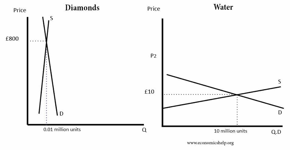